


Imagine you're tasked with presenting monthly sales performance to your company's leadership team. The data includes thousands of transactions across multiple regions, products, and sales representatives. Simply sharing raw data wouldn't suffice--it's overwhelming and obscures the key insights you want to convey. What's needed is a clear, organized summary that highlights key metrics like total sales by region, top-performing products, and individual contributions. This is where tabular reports come into play.

Imagine you're tasked with presenting monthly sales performance to your company's leadership team. The data includes thousands of transactions across multiple regions, products, and sales representatives. Simply sharing raw data wouldn't suffice--it's overwhelming and obscures the key insights you want to convey. What's needed is a clear, organized summary that highlights key metrics like total sales by region, top-performing products, and individual contributions. This is where tabular reports come into play.
Sorting Datasets Using PROC SORT
In SAS programming, sorting data serves several purposes: organizing it for reports, preparing datasets for merging, or enabling the use of a BY statement in another PROC or DATA step. As the name suggests, PROC SORT sorts observations based on the variables in its BY statement (and thereby the BY statement is required for PROC SORT).
PROC SORT DATA=<dataset_name>; BY <variable-list>;RUN;
For example, let's consider sorting the dataset created by the following DATA step:
DATA customer_order; INPUT customer_name &$10. amount order_date; DATALINES;John Doe 89.99 2023-11-25Jane Smith 45.50 2023-12-01Bob Lee 120.00 2023-12-10Mark Tao 35.75 2023-12-15Mark Tao 150.25 2023-12-20;RUN;
The dataset includes one character variable (customer_name), one numeric variable (amount), and one date variable (order_date). Now, let's first sort this dataset by amount:
PROC SORT DATA=customer_order;    BY amount;RUN;
PROC PRINT DATA=customer_order;RUN;

Observe that the data is sorted by amount in an ascending order. By default, PROC SORT arranges data in ascending order. To sort in descending order, include the keyword DESCENDING before the name of the BY variable:
PROC SORT DATA=customer_order;    BY DESCENDING amount;RUN;
PROC PRINT DATA=customer_order;RUN;

If there are more than one variable is specified in the BY statement, SAS sorts observations by the first variable, then by the second variable within the same value of the first variable, and so on. For example:
PROC SORT DATA=customer_order;        /* Sort by customer_name and then amount */    BY customer_name DESCENDING amount;RUN;
PROC PRINT DATA=customer_order;RUN;

Here, SAS sorts first by customer_name in alphabetical order (A to Z) and then sorts by amount in descending order within each customer_name group. So, for the same customer_name values (e.g., Mark Tao in the 4th and 5th observation), the observations are sorted based on the amount.
Internally, SAS converts date values to the number of days since January 1, 1960. So essentially, sorting by a date variable works in the same way as sorting by a numeric variable. For example:
PROC SORT DATA=customer_order;    BY order_date;RUN;
PROC PRINT DATA=customer_order;RUN;

In this example, the dataset is sorted by the order_date variable in an ascending order. As mentioned earlier, the numbers contained in the order_date represent the number of days since January 1, 1960. Therefore, the older dates appear first when the data is sorted in ascending order.
In SAS programming, sorting data serves several purposes: organizing it for reports, preparing datasets for merging, or enabling the use of a BY statement in another PROC or DATA step. As the name suggests, PROC SORT sorts observations based on the variables in its BY statement (and thereby the BY statement is required for PROC SORT).
PROC SORT DATA=<dataset_name>;BY <variable-list>;RUN;
For example, let's consider sorting the dataset created by the following DATA step:
DATA customer_order;INPUT customer_name &$10. amount order_date;DATALINES;John Doe 89.99 2023-11-25Jane Smith 45.50 2023-12-01Bob Lee 120.00 2023-12-10Mark Tao 35.75 2023-12-15Mark Tao 150.25 2023-12-20;RUN;
The dataset includes one character variable (customer_name), one numeric variable (amount), and one date variable (order_date). Now, let's first sort this dataset by amount:
PROC SORT DATA=customer_order;BY amount;RUN;PROC PRINT DATA=customer_order;RUN;

Observe that the data is sorted by amount in an ascending order. By default, PROC SORT arranges data in ascending order. To sort in descending order, include the keyword DESCENDING before the name of the BY variable:
PROC SORT DATA=customer_order;BY DESCENDING amount;RUN;PROC PRINT DATA=customer_order;RUN;

If there are more than one variable is specified in the BY statement, SAS sorts observations by the first variable, then by the second variable within the same value of the first variable, and so on. For example:
PROC SORT DATA=customer_order;/* Sort by customer_name and then amount */BY customer_name DESCENDING amount;RUN;PROC PRINT DATA=customer_order;RUN;

Here, SAS sorts first by customer_name in alphabetical order (A to Z) and then sorts by amount in descending order within each customer_name group. So, for the same customer_name values (e.g., Mark Tao in the 4th and 5th observation), the observations are sorted based on the amount.
Internally, SAS converts date values to the number of days since January 1, 1960. So essentially, sorting by a date variable works in the same way as sorting by a numeric variable. For example:
PROC SORT DATA=customer_order;BY order_date;RUN;PROC PRINT DATA=customer_order;RUN;

In this example, the dataset is sorted by the order_date variable in an ascending order. As mentioned earlier, the numbers contained in the order_date represent the number of days since January 1, 1960. Therefore, the older dates appear first when the data is sorted in ascending order.
PROC SORT Options
Controlling the Output Dataset
Unlike DATA steps, which create a new SAS dataset without modifying the original input data source specified in the SEST or INFILE statement, certain PROC steps can alter the input data. This is because essentially PROC steps are designed to process the input data directly, rather than creating a separate output dataset. PROC SORT is an example of such a procedure, as it modifies the specified dataset, by rearranging its observations. For example:
DATA air_quality;    INPUT date :YYMMDD10. pm25 no2 o3_level status $10.;    DATALINES;2023-12-01 10.5 45 32 Moderate2023-12-02 15.2 50 28 Unhealthy2023-12-03 8.0 35 40 Good2023-12-04 20.1 55 25 Unhealthy2023-12-05 12.3 42 30 Moderate;RUN;
/* Print data before applying PROC SORT */PROC PRINT DATA=air_quality;    TITLE 'Before PROC SORT';RUN;
PROC SORT DATA=air_quality;    BY pm25;RUN;
/* Print data after applying PROC SORT */PROC PRINT DATA=air_quality;    TITLE 'After PROC SORT';RUN;

To avoid modifying the input dataset and save the PROC results as a separate dataset, use the OUT= option in the PROC statement. This option specifies a new output dataset for the sorted results. For example:
DATA air_quality;    INPUT date :YYMMDD10. pm25 no2 o3_level status $10.;    DATALINES;2023-12-01 10.5 45 32 Moderate2023-12-02 15.2 50 28 Unhealthy2023-12-03 8.0 35 40 Good2023-12-04 20.1 55 25 Unhealthy2023-12-05 12.3 42 30 Moderate;RUN;
PROC SORT DATA=air_quality OUT=sorted_air_quality;    BY pm25;RUN;
/* Print original data */PROC PRINT DATA=air_quality;    TITLE 'Original data';RUN;
/* Print sorted data */PROC PRINT DATA=sorted_air_quality;    TITLE 'Sorted data';RUN;

Unlike DATA steps, which create a new SAS dataset without modifying the original input data source specified in the SEST or INFILE statement, certain PROC steps can alter the input data. This is because essentially PROC steps are designed to process the input data directly, rather than creating a separate output dataset. PROC SORT is an example of such a procedure, as it modifies the specified dataset, by rearranging its observations. For example:
DATA air_quality;INPUT date :YYMMDD10. pm25 no2 o3_level status $10.;DATALINES;2023-12-01 10.5 45 32 Moderate2023-12-02 15.2 50 28 Unhealthy2023-12-03 8.0 35 40 Good2023-12-04 20.1 55 25 Unhealthy2023-12-05 12.3 42 30 Moderate;RUN;/* Print data before applying PROC SORT */PROC PRINT DATA=air_quality;TITLE 'Before PROC SORT';RUN;PROC SORT DATA=air_quality;BY pm25;RUN;/* Print data after applying PROC SORT */PROC PRINT DATA=air_quality;TITLE 'After PROC SORT';RUN;

To avoid modifying the input dataset and save the PROC results as a separate dataset, use the OUT= option in the PROC statement. This option specifies a new output dataset for the sorted results. For example:
DATA air_quality;INPUT date :YYMMDD10. pm25 no2 o3_level status $10.;DATALINES;2023-12-01 10.5 45 32 Moderate2023-12-02 15.2 50 28 Unhealthy2023-12-03 8.0 35 40 Good2023-12-04 20.1 55 25 Unhealthy2023-12-05 12.3 42 30 Moderate;RUN;PROC SORT DATA=air_quality OUT=sorted_air_quality;BY pm25;RUN;/* Print original data */PROC PRINT DATA=air_quality;TITLE 'Original data';RUN;/* Print sorted data */PROC PRINT DATA=sorted_air_quality;TITLE 'Sorted data';RUN;

Removing Duplicates
When analyzing data, it is often necessary to identify the unique values within a particular variable. This information is essential for tasks such as data cleaning, feature engineering, and exploratory data analysis.
In SAS, the NODUPKEY option used with the PROC SORT can be used for the purpose. For example, the sashelp.baseball dataset contains 322 MLB players who played at least one game during the 1986--1987 seasons across 24 teams. Let's explore how to identify the unique teams included in the team variable. As we discussed earlier, using PROC SORT by default modifies the original dataset. To prevent this in our example, we'll specify the OUT= option. This creates a new dataset, baseball_team, containing only unique team names from the sashelp.baseball dataset.
PROC SORT DATA=sashelp.baseball OUT=baseball_team NODUPKEY;    BY team;RUN;
/* Print the unique list of baseball teams in SAS log */DATA _null_;
    SET baseball_team;    PUT team;RUN;
Atlanta Baltimore Boston California Chicago Cincinnati Cleveland Detroit Houston Kansas City Los Angeles Milwaukee Minneapolis Montreal New York Oakland Philadelphia Pittsburgh San Diego San Francisco Seattle St Louis Texas Toronto NOTE: There were 24 observations read from the data set WORK.BASEBALL_TEAM.In some cases, you might also want to retain the observations containing duplicate values in a separate dataset. When used in conjunction with the NODUPKEY option, the DUPOUT= option within the PROC SORT statement creates a separate dataset containing all observations that have duplicate values for the specified BY variables. For example:
PROC SORT DATA=sashelp.baseball OUT=baseball_team NODUPKEY DUPOUT=dup_obs;    BY team;RUN;
/* Print the first 15 observations of the duplicated data */PROC PRINT DATA=dup_obs (OBS=15);RUN;

When analyzing data, it is often necessary to identify the unique values within a particular variable. This information is essential for tasks such as data cleaning, feature engineering, and exploratory data analysis.
In SAS, the NODUPKEY option used with the PROC SORT can be used for the purpose. For example, the sashelp.baseball dataset contains 322 MLB players who played at least one game during the 1986--1987 seasons across 24 teams. Let's explore how to identify the unique teams included in the team variable. As we discussed earlier, using PROC SORT by default modifies the original dataset. To prevent this in our example, we'll specify the OUT= option. This creates a new dataset, baseball_team, containing only unique team names from the sashelp.baseball dataset.
PROC SORT DATA=sashelp.baseball OUT=baseball_team NODUPKEY;BY team;RUN;/* Print the unique list of baseball teams in SAS log */DATA _null_;SET baseball_team;PUT team;RUN;
In some cases, you might also want to retain the observations containing duplicate values in a separate dataset. When used in conjunction with the NODUPKEY option, the DUPOUT= option within the PROC SORT statement creates a separate dataset containing all observations that have duplicate values for the specified BY variables. For example:
PROC SORT DATA=sashelp.baseball OUT=baseball_team NODUPKEY DUPOUT=dup_obs;BY team;RUN;/* Print the first 15 observations of the duplicated data */PROC PRINT DATA=dup_obs (OBS=15);RUN;

Setting Character Sort Order
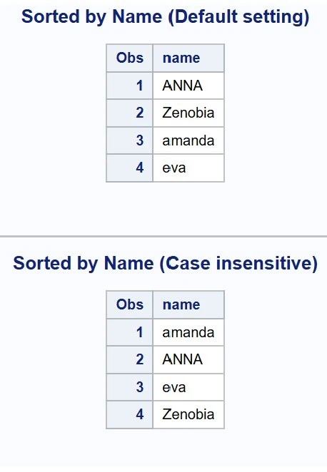
When sorting observations by character variables, you can explicitly specify a collating sequence rather than relying on the default settings. A commonly used collating sequence in PROC SORT is SORTSEQ=LINGUISTIC with the (STRENGTH=PRIMARY) suboption. This tells SAS to sort the character values, ignoring the case. For example:
DATA example_data;    INPUT name $;    DATALINES;evaamandaZenobiaANNARUN;
PROC SORT DATA=example_data OUT=default_setting;    BY name;RUN;
PROC SORT DATA=example_data OUT=case_insensitive SORTSEQ=LINGUISTIC (STRENGTH=PRIMARY);     BY name;RUN;
PROC PRINT DATA=default_setting;    TITLE "Sorted by Name (Default setting)";RUN;
PROC PRINT DATA=case_insensitive;    TITLE "Sorted by Name (Case insensitive)";RUN;
Occasionally, numeral values are stored as character values. When applying PROC SORT to such values, it sorts data as if they are character strings. So, for example, the value "10" comes before "2". However, (NUMERIC_COLLATION=ON) suboption along with the SORTSEQ=LINGUISTIC option tells SAS to treat numerals as their numeric equivalents. This is particularly useful when the BY variable is mixed with numbers and characters. For example:
DATA example_data2;    INPUT name $ 1-8 competitions $ 9-25;    DATALINES;eva     1500m freestyleamanda  200m breaststrokeZenobia 100m backstrokeANNA    50m freestyle;RUN;
/* Sorts data without suboption */PROC SORT DATA=example_data2 OUT=sort_by_default;    BY competitions;RUN;
/* Sorts data with numeric collation option */PROC SORT DATA=example_data2 OUT=sort_by_numeric SORTSEQ=LINGUISTIC (NUMERIC_COLLATION=ON);    BY Competitions;RUN;
/* Print sorted data (default) */PROC PRINT DATA=sort_by_default;    TITLE "Sorted by Competitions (Default)";RUN;
/* Print sorted data (numeric collation) */PROC PRINT DATA=sort_by_numeric;    TITLE "Sorted by Competitions (Numeric collation)";RUN;

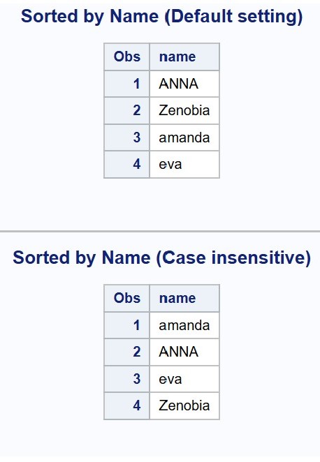
When sorting observations by character variables, you can explicitly specify a collating sequence rather than relying on the default settings. A commonly used collating sequence in PROC SORT is SORTSEQ=LINGUISTIC with the (STRENGTH=PRIMARY) suboption. This tells SAS to sort the character values, ignoring the case. For example:
DATA example_data;INPUT name $;DATALINES;evaamandaZenobiaANNARUN;PROC SORT DATA=example_data OUT=default_setting;BY name;RUN;PROC SORT DATA=example_data OUT=case_insensitive SORTSEQ=LINGUISTIC (STRENGTH=PRIMARY);BY name;RUN;PROC PRINT DATA=default_setting;TITLE "Sorted by Name (Default setting)";RUN;PROC PRINT DATA=case_insensitive;TITLE "Sorted by Name (Case insensitive)";RUN;
Occasionally, numeral values are stored as character values. When applying PROC SORT to such values, it sorts data as if they are character strings. So, for example, the value "10" comes before "2". However, (NUMERIC_COLLATION=ON) suboption along with the SORTSEQ=LINGUISTIC option tells SAS to treat numerals as their numeric equivalents. This is particularly useful when the BY variable is mixed with numbers and characters. For example:
DATA example_data2;INPUT name $ 1-8 competitions $ 9-25;DATALINES;eva 1500m freestyleamanda 200m breaststrokeZenobia 100m backstrokeANNA 50m freestyle;RUN;/* Sorts data without suboption */PROC SORT DATA=example_data2 OUT=sort_by_default;BY competitions;RUN;/* Sorts data with numeric collation option */PROC SORT DATA=example_data2 OUT=sort_by_numeric SORTSEQ=LINGUISTIC (NUMERIC_COLLATION=ON);BY Competitions;RUN;/* Print sorted data (default) */PROC PRINT DATA=sort_by_default;TITLE "Sorted by Competitions (Default)";RUN;/* Print sorted data (numeric collation) */PROC PRINT DATA=sort_by_numeric;TITLE "Sorted by Competitions (Numeric collation)";RUN;

Customizing Sort Orders with PROC FORMAT
Let's revisit the air_quality dataset mentioned earlier:
DATA air_quality; INPUT date :YYMMDD10. pm25 no2 o3_level status $10.; DATALINES;2023-12-01 10.5 45 32 Moderate2023-12-02 15.2 50 28 Unhealthy2023-12-03 8.0 35 40 Good2023-12-04 20.1 55 25 Unhealthy2023-12-05 12.3 42 30 Moderate;RUN;
In the dataset, observe that the status values--Unhealthy, Moderate, and Good--has a natural order. Categorical data with such inherent ordering is referred to as ordinal data. To sort ordinal data by their order rather than alphabetically, you can use the PROC FORMAT like:
PROC FORMAT;    VALUE $airqfmt        'Unhealthy' = 1        'Moderate' = 2        'Good' = 3;RUN;
DATA sorted_data;    SET air_quality;    airq_order = PUT(status, $airqfmt.);RUN;
PROC SORT DATA=sorted_data;    BY airq_order;RUN;
PROC PRINT DATA=sorted_data;RUN;

PROC FORMAT creates custom formats for data values that can later be used in the subsequent DATA or PROC steps. These formats define how data is read, transforming your data more suitable for your data analysis.
The basic syntax of the PROC FORMAT is:
PROC FORMAT; VALUE [$]format-name data-value-1 = 'Label 1' data-value-2 = 'Label 2' ⠇ data-value-N = 'Label N';RUN;
The VALUE statement defines the name of the format you're creating, as well as the mapping between data values and their corresponding labels. The name should be descriptive and adhere to the following rules:
- Length:
- Character Formats: Up to 31 characters.
- Numeric Formats: Up to 32 characters.
- First Character:
- Character Formats: Must begin with a dollar sign ($).
- Numeric Formats: Must begin with a letter (A-Z, a-z) or an underscore (_)
- Subsequent Characters: Can be letters, numbers (0-9), or underscores (_). Any other special characters or blank space are not allowed.
- Reserved Names: Avoid using names reserved by SAS for automatic variables, variable lists, datasets, and librefs.
Just like any other SAS language element, formats are case-insensitive. For example, $airqformat, $AirqFmt, and $AIRQFMT are considered the same format element.
Created SAS formats can then be used interchangeably with pre-defined formats, providing the same flexibility in reading, displaying and transforming data values. One common way to apply specific formats to data is using the PUT function:
PUT(source, format.)
In SAS, the period (.) following the element name in the PUT function (or anywhere else it is applied) is used to indicate that the specified element is a format.
Let's revisit the air_quality dataset mentioned earlier:
DATA air_quality;INPUT date :YYMMDD10. pm25 no2 o3_level status $10.;DATALINES;2023-12-01 10.5 45 32 Moderate2023-12-02 15.2 50 28 Unhealthy2023-12-03 8.0 35 40 Good2023-12-04 20.1 55 25 Unhealthy2023-12-05 12.3 42 30 Moderate;RUN;
In the dataset, observe that the status values--Unhealthy, Moderate, and Good--has a natural order. Categorical data with such inherent ordering is referred to as ordinal data. To sort ordinal data by their order rather than alphabetically, you can use the PROC FORMAT like:
PROC FORMAT;VALUE $airqfmt'Unhealthy' = 1'Moderate' = 2'Good' = 3;RUN;DATA sorted_data;SET air_quality;airq_order = PUT(status, $airqfmt.);RUN;PROC SORT DATA=sorted_data;BY airq_order;RUN;PROC PRINT DATA=sorted_data;RUN;

PROC FORMAT creates custom formats for data values that can later be used in the subsequent DATA or PROC steps. These formats define how data is read, transforming your data more suitable for your data analysis.
The basic syntax of the PROC FORMAT is:
PROC FORMAT;VALUE [$]format-namedata-value-1 = 'Label 1'data-value-2 = 'Label 2'⠇data-value-N = 'Label N';RUN;
The VALUE statement defines the name of the format you're creating, as well as the mapping between data values and their corresponding labels. The name should be descriptive and adhere to the following rules:
- Length:
- Character Formats: Up to 31 characters.
- Numeric Formats: Up to 32 characters.
- First Character:
- Character Formats: Must begin with a dollar sign ($).
- Numeric Formats: Must begin with a letter (A-Z, a-z) or an underscore (_)
- Subsequent Characters: Can be letters, numbers (0-9), or underscores (_). Any other special characters or blank space are not allowed.
- Reserved Names: Avoid using names reserved by SAS for automatic variables, variable lists, datasets, and librefs.
Just like any other SAS language element, formats are case-insensitive. For example, $airqformat, $AirqFmt, and $AIRQFMT are considered the same format element.
Created SAS formats can then be used interchangeably with pre-defined formats, providing the same flexibility in reading, displaying and transforming data values. One common way to apply specific formats to data is using the PUT function:
PUT(source, format.)
In SAS, the period (.) following the element name in the PUT function (or anywhere else it is applied) is used to indicate that the specified element is a format.
Aside: Grouping Observations Using PROC FORMAT
The PROC FORMAT can also be used to group and re-categorize the data values. For example:
DATA age_data;    INPUT first_name $ last_name $ age;    DATALINES;Alice Smith 23Bob Johnson 45Charlie Williams 12David Brown 67Eva Davis 34Frank Miller 56Grace Wilson 18Hannah Moore 29Ian Taylor 60Jack Anderson 72;RUN;
PROC FORMAT;    VALUE agefmt        LOW - 18 = 'Underage' /* Values from the lowest possible to 18 (inclusive) */        18 <- 40 = 'Young Adult' /* Values from 19 to 40 */        40 -< 65 = 'Adult' /* Values from 41 to 64 */        65 - HIGH = 'Senior'; /* Catch-all for values outside the defined ranges */ RUN;
DATA categorized_data;    SET age_data;    age_group = PUT(age, agefmt.);RUN;
PROC PRINT DATA=categorized_data;RUN;

In this example, the age values are grouped by a categorical range. The range specification is done by dash (-). The LOW and HIGH keyword represent the smallest and largest possible values, respectively.
Note that the ranges specified with the dash sign is inclusive. For example, LOW - 18 captures all the values from the lowest up to and including 18. Similarly, 65 - HIGH captures value from 65 to the largest possible. To represent an exclusive range, you can use the less than sign (<). If you are excluding the first value in a range, then put the less than sign after the value. For example, 18 <- 40 in the code above does not include the value of 18. Similarly, if you are excluding the last value in the range, then put the less than sign before the range. For example, 40 -< 65 does not include the value of 65, so that there is no overlapping ranges.
To group values within a character variable, you can assign the same label to more than one data values within the VALUE statement of a PROC FORMAT. Use commas (,) to separate the individual data values that should be assigned to the same label on the left side of the equal sign.
PROC FORMAT; VALUE $airqfmt 'Unhealthy', 'Moderate' = 1 'Good' = 2 OTHER = 3; RUN;
The keyword OTHER can be used to assign a default label or value to any data values that do not match any of the explicitly defined values in the VALUE statement. In the example above, OTHER = 3 means that any value not equal to 'Unhealthy', 'Moderate', or 'Good' will be assigned the value 3. So in this case, if a future observation can potentially include values like 'Excellent' or 'Poor' that aren't listed in the VALUE statement, they will automatically be assigned the value 3.
The PROC FORMAT can also be used to group and re-categorize the data values. For example:
DATA age_data;INPUT first_name $ last_name $ age;DATALINES;Alice Smith 23Bob Johnson 45Charlie Williams 12David Brown 67Eva Davis 34Frank Miller 56Grace Wilson 18Hannah Moore 29Ian Taylor 60Jack Anderson 72;RUN;PROC FORMAT;VALUE agefmtLOW - 18 = 'Underage' /* Values from the lowest possible to 18 (inclusive) */18 <- 40 = 'Young Adult' /* Values from 19 to 40 */40 -< 65 = 'Adult' /* Values from 41 to 64 */65 - HIGH = 'Senior'; /* Catch-all for values outside the defined ranges */RUN;DATA categorized_data;SET age_data;age_group = PUT(age, agefmt.);RUN;PROC PRINT DATA=categorized_data;RUN;

In this example, the age values are grouped by a categorical range. The range specification is done by dash (-). The LOW and HIGH keyword represent the smallest and largest possible values, respectively.
Note that the ranges specified with the dash sign is inclusive. For example, LOW - 18 captures all the values from the lowest up to and including 18. Similarly, 65 - HIGH captures value from 65 to the largest possible. To represent an exclusive range, you can use the less than sign (<). If you are excluding the first value in a range, then put the less than sign after the value. For example, 18 <- 40 in the code above does not include the value of 18. Similarly, if you are excluding the last value in the range, then put the less than sign before the range. For example, 40 -< 65 does not include the value of 65, so that there is no overlapping ranges.
To group values within a character variable, you can assign the same label to more than one data values within the VALUE statement of a PROC FORMAT. Use commas (,) to separate the individual data values that should be assigned to the same label on the left side of the equal sign.
PROC FORMAT;VALUE $airqfmt'Unhealthy', 'Moderate' = 1'Good' = 2OTHER = 3;RUN;
The keyword OTHER can be used to assign a default label or value to any data values that do not match any of the explicitly defined values in the VALUE statement. In the example above, OTHER = 3 means that any value not equal to 'Unhealthy', 'Moderate', or 'Good' will be assigned the value 3. So in this case, if a future observation can potentially include values like 'Excellent' or 'Poor' that aren't listed in the VALUE statement, they will automatically be assigned the value 3.
Aside: Encoding and Decoding Data Using PROC FORMAT
In the context of data analysis, data encoding refers to the process of transforming categorical data into numerical representations. This technique makes it easier to apply statistical models or machine learning algorithms requiring numerical inputs.
In SAS, you can use PROC FORMAT for the purpose:
PROC FORMAT;    VALUE $sexfmt        'Male' = 0         'Female' = 1;RUN;
/* Dataset with formatted sex */DATA mydata;    INPUT sex $ height weight;    encoded_sex = INPUT(PUT(sex, $sexfmt.), 1.);    DATALINES;Male   180 75Female 165 60Male   175 80Female 160 55Male   185 90Female 155 50Male   178 85Female 162 58Male   172 78Female 168 65;RUN;
/* Regression using the formatted values */PROC REG DATA=mydata;    MODEL height = encoded_sex weight;    ODS SELECT ParameterEstimates;RUN;

On the other hand, data decoding refers to the process of converting encoded data back into the meaningful form. This is commonly involved when working with survey data, where coded values represent specific categories or responses for each questions (e.g., "1" for "Yes" and "2" for "No"). Decoding translates these codes into human-readable form, making the data easier to interpret and analyze. For example:
DATA survey_response;    INPUT name $ response $ rating $;    DATALINES;John  1 5Sarah 2 4Tom   1 2Alice 2 3;RUN;
PROC PRINT DATA=survey_response;RUN;

As shown in the PROC PRINT results above, interpreting the raw responses without a codebook is difficult because the numerical values do not immediately convey meaningful information. Also, the same value can represent different meanings depending on the question (e.g., 1 has different meaning for response and rating).
To make the data more interpretable, we can apply the formats defined by PROC FORMAT. This transformation makes the raw data values clearer and easier to understand:
PROC FORMAT;
    VALUE $responsefmt
         1 = 'Yes'
         2 = 'No';
    VALUE $ratingfmt
        5 = 'Excellent'
        4 = 'Good'
        3 = 'Average'
        2 = 'Poor'
        1 = 'Very Poor';
RUN;
DATA decoded_response;    SET survey_response;        /* Decode responses using the formats */    response = PUT(response, responsefmt.);    rating = PUT(rating, ratingfmt.);  RUN;
PROC PRINT DATA=decoded_response;RUN;

In the context of data analysis, data encoding refers to the process of transforming categorical data into numerical representations. This technique makes it easier to apply statistical models or machine learning algorithms requiring numerical inputs.
In SAS, you can use PROC FORMAT for the purpose:
PROC FORMAT;VALUE $sexfmt'Male' = 0'Female' = 1;RUN;/* Dataset with formatted sex */DATA mydata;INPUT sex $ height weight;encoded_sex = INPUT(PUT(sex, $sexfmt.), 1.);DATALINES;Male 180 75Female 165 60Male 175 80Female 160 55Male 185 90Female 155 50Male 178 85Female 162 58Male 172 78Female 168 65;RUN;/* Regression using the formatted values */PROC REG DATA=mydata;MODEL height = encoded_sex weight;ODS SELECT ParameterEstimates;RUN;

On the other hand, data decoding refers to the process of converting encoded data back into the meaningful form. This is commonly involved when working with survey data, where coded values represent specific categories or responses for each questions (e.g., "1" for "Yes" and "2" for "No"). Decoding translates these codes into human-readable form, making the data easier to interpret and analyze. For example:
DATA survey_response;INPUT name $ response $ rating $;DATALINES;John 1 5Sarah 2 4Tom 1 2Alice 2 3;RUN;PROC PRINT DATA=survey_response;RUN;

As shown in the PROC PRINT results above, interpreting the raw responses without a codebook is difficult because the numerical values do not immediately convey meaningful information. Also, the same value can represent different meanings depending on the question (e.g., 1 has different meaning for response and rating).
To make the data more interpretable, we can apply the formats defined by PROC FORMAT. This transformation makes the raw data values clearer and easier to understand:
PROC FORMAT; VALUE $responsefmt 1 = 'Yes' 2 = 'No'; VALUE $ratingfmt 5 = 'Excellent' 4 = 'Good' 3 = 'Average' 2 = 'Poor' 1 = 'Very Poor'; RUN;DATA decoded_response;SET survey_response;/* Decode responses using the formats */response = PUT(response, responsefmt.);rating = PUT(rating, ratingfmt.);RUN;PROC PRINT DATA=decoded_response;RUN;

Listing Observations with PROC PRINT
In the examples we've seen so far, we used PROC PRINT to display observations from SAS datasets. The PRINT procedure outputs the dataset, potentially with the following options:
- (OBS=n): This suboption prints out only the first n observations from the beginning. Note that the (OBS=n) suboption must be used prior to NOOBS and LABEL.
- NOOBS: By default, the PRINT procedure the observation numbers along side the variables. If you don't want the observation numbers, however, you can use the NOOBS option.
- LABEL: Allows you to use variable labels instead of variable names in the output. Should be used with the LABEL statement in the procedure.
Additionally, the following statements can also be used:
- BY variable-list: Starts a new section in the result for each new value of the BY variables. Note that the data must be presorted by the BY variables in ascending order.
- ID variable-list: Use the ID variable instead of the default OBS numbers on the left-hand side of the printed output.
- SUM variable-list: Sums for the variables in the list. If used with the BY statement, it shows the sum of the specified variable by each BY variable value, as well as the total sum.
- VAR variable-list: Specifies which variables to print and the order. Without a VAR statement, all variables in the SAS dataset are printed in the order that they occur in the dataset.
The following example shows all these options together:
PROC SORT DATA=sashelp.baseball OUT=sort_by_team;    BY team;RUN;
PROC PRINT DATA=sort_by_team (OBS=26) NOOBS LABEL;    VAR nAtBat nHits nHome nRBI Name;    LABEL nAtBat = 'Number of Times Batted'          nHits = 'Number of Hits'          nHome = 'Number of Home Runs'          nRBI = 'Number of Run Batted in'          nBB = 'Number of Base on Balls';    BY team;    SUM nAtBat nHits nHome nRBI nBB;RUN;

When listing observations using the PROC PRINT, the FORMAT statement changes the appearance of the data values.
- For numeric values, you can specify a format along with the width w and decimals d (formatw.d). It is worth noting that the period (.) and d also counts for w. For example, FORMAT my_var 5.3; can display the values up to 9.999. Similarly, FORMAT my_var 1.0; can display the values up to 9.0. Any values exceeding it will be displayed as an asterisk (*).
- For character values, you must put a dollar sign to indicate that it is character format ($formatw.). Character formats take only the width w.
- Date formats converts the SAS date (the number of days since Jan 1, 1960 to the date value) into the specified format and display the converted date.
Here are some commonly used SAS standard formats:
Informat Width Input Data INPUT Statement Results Character $UPCASEw.
Converts character data to uppercase. 1-32767 (default: 8 or variable length) John Doe FORMAT name $UPCASE10.; JOHN DOE $w.
Writes standard character data,
while maintaining leading blanks. 1-32767
(default: 1 or variable length) John Doe
Jane Doe FORMAT name $9.; John Doe
Jane Do Date, Time, and Datetime DATEw.
Writes SAS dates in form:
ddmmmyy
or ddmmmyyyy 5-11 (default: 7) 18966 FORMAT my_date DATE7.;
FORMAT my_date DATE9.; 05DEC11
05DEC2011 DATETIMEw.
Writes SAS datetimes in form:
ddmmmyy hh:mm:ss.ss 7-40 (default: 16) 26530 FORMAT my_dt DATETIME13.;
FORMAT my_dt DATETIME18.1; 01JAN60:07:22
01JAN60:07:22:10.0 DTDATEw.
Writes SAS datetimes in from:
ddmmyy
or ddmmyyyy 5-9 (default: 7) 26530 FORMAT my_dt DTDATE7.;
FORMAT my_dt DTDATE9.; 01JAN60
01JAN1960 EURDFDDw.
Writes SAS dates in form:
dd.mm.yy
or dd.mm.yyyy 2-10 (default: 8) 18966 FORMAT my_date EURDFDD8.;
FORMAT my_date EURDFDD10.; 05.12.11
05.12.2011 JULIANw.
Writes SAS dates in Julian form:
yyddd
or yyyyddd 5-7 (default: 5) 18966 FORMAT my_date JULIAN5.;
FORMAT my_date JULIAN7.; 11339
2011339 MMDDYYw.
Writes SAS dates in form:
mmddyy
or mm/dd/yyyy 2-10 (default: 8) 18966 FORMAT my_date MMDDYY6.;
FORMAT my_date MMDDYY8.; 120511
12/05/11 TIMEw.d
Writes SAS time in form:
hh:mm:ss.ss 2-20 (default: 8) 26530 FORMAT my_time TIME8.;
FORMAT my_time TIME11.2; 7:22:10
7:22:10.00 WEEKDATEw.
Writes SAS date in form:
day-of-week,
month-name dd,
yy, or yyyy 3-37 (default: 29) 18966 FORMAT my_date WEEKDATE15.;
Mon, Dec 5, 11
WORDDATEw.
Writes SAS dates in form:
month-name dd, yyyy 3-32 (default: 18) 18966 FORMAT my_date WORDDATE12.;
FORMAT my_date WORDDATE18.; Dec 5, 2011
December 5, 2011 Numeric BESTw.
SAS determines best format for data. 1-32 (default: 12) 1200001 FORMAT my_num BEST6.;
FORMAT my_num BEST8.; 1.20E6
1200001 COMMAw.d
Writes numbers with commas. 2-32 (default: 6) 1200001 FORMAT my_num COMMA9.;
FORMAT my_num COMMA12.2; 1,200,001
1,200,001.00 DOLLARw.d
Writes numbers with a leading $ and commas. 2-32 (default: 6) 1200001 FORMAT my_num DOLLAR10.;
FORMAT my_num DOLLAR13.2; $1,200,001
$1,200,001.00 Ew.
Writes numbers in scientific notation. 7-32 (default: 12)
1200001
FORMAT my_num E7.; 1.2E+06 EUROXw.d
Writes numbers with a leading € and periods. 2-32 (default: 6) 1200001
FORMAT my_num EUROX13.2; €1.200.001,00 PERCENTw.d
Writes numeric data as percentage. 4-32 (default: 6) 0.05 FORMAT my_num PERCENT9.2; 5.00% w.d
Writes standard numeric data. 1-32 12.345 FORMAT my_num 6.2;
FORMAT my_num 5.2; 12.345
12.35
For example:
DATA customer_order;    INPUT customer_name &$20. amount order_date :YYMMDD10.;    DATALINES;John Doe    89.99   2023-11-25Jane Smith  45.50   2023-12-01Bob Lee     120.00  2023-12-10Mark Tao    35.75   2023-12-15Mark Tao    150.25  2023-12-20RUN;
PROC PRINT DATA=customer_order;    FORMAT        customer_name $UPPERCASE20.        amount DOLLAR8.2        order_date WEEKDATE29.;RUN;

Of course, you can also apply custom data formats created using PROC FORMAT. For example:
PROC FORMAT;    VALUE amountfmt        LOW - 40 = '$'        41 - 80 = '$$'        81 - 120 = '$$$'        121 - HIGH = '$$$$';RUN;
PROC PRINT DATA=customer_order;    FORMAT         amount amountfmt.        order_date WEEKDATE29.;RUN;

[1] Format names can be up to 32 characters in length and can contain letters, numbers, and underscores. The first character of the name must be a letter ↩
Tabular reports transform raw data into structured, digestible tables that provide actionable insights at a glance. By aggregating, summarizing, and organizing key metrics into rows and columns, they allows you to extract information from your data and present concisely, helping decision-making process.
This tutorial will guide you through creating these reports using SAS. We will start by calculating summary statistics with PROC MEANS and creating frequency distribution tables using PROC FREQ. Next, we'll explore creating professional-grade reports with PROC TABULATE.
This tutorial uses a dataset created by the following DATA step:
DATA sales_data;    INPUT  txn_date :MMDDYY10. region $ prod $ rep $ price qs;
    FORMAT txn_date  MMDDYY10.;    LABEL        txn_date = "Transaction Date"        region = "Sales Region"        prod = "Product Type"        rep = "Sales Representative"        price = "Unit Price (USD)"        qs = "Quantity Sold";
    DATALINES;
01/02/2024 North Laptop Alice   1500 2
01/05/2024 North Tablet Alice   750  3
01/08/2024 South Laptop Bob     1700 1
01/12/2024 East  Tablet Charlie 800  .
01/15/2024 West  Laptop David   1800 2
01/18/2024 North Tablet Alice   780  2
01/22/2024 South Laptop Bob     1650 1
01/25/2024 East  Tablet Charlie 850  3
01/28/2024 West  Laptop David   1900 .
02/01/2024 North Laptop Alice   1550 2
02/03/2024 South Tablet Bob     720  5
02/07/2024 East  Laptop Charlie 1600 1
02/10/2024 West  Tablet David   820  2
02/12/2024 North Laptop Alice   .    3
02/15/2024 South Laptop Bob     .    2
02/18/2024 East  Tablet Charlie 880  1
02/21/2024 West  Laptop David   1950 2
02/24/2024 North Tablet Alice   .    4
02/27/2024 South Laptop Bob     1590 2
03/01/2024 East  Tablet Charlie 900  3
03/03/2024 West  Laptop David   1850 1
03/06/2024 North Tablet Alice   770  5
03/08/2024 South Laptop Bob     1600 2
03/11/2024 East  Tablet .       .    1
03/14/2024 West  Laptop David   1920 2
03/17/2024 North Laptop Alice   1580 1
03/20/2024 South Tablet Bob     740  3
03/23/2024 East  Laptop Charlie 1620 2
03/25/2024 West  Tablet David   860  4
;
RUN;
PROC CONTENTS DATA=sales_data;    ODS SELECT Variables;RUN;

This dataset contains monthly sales transaction records across four regions (North, South, East, and West) for two product types (Laptops and Tablets). Each record details a single sales transaction and includes: transaction date, sales region, product type, sales representative, unit price, quantity sold.
In the examples we've seen so far, we used PROC PRINT to display observations from SAS datasets. The PRINT procedure outputs the dataset, potentially with the following options:
- (OBS=n): This suboption prints out only the first n observations from the beginning. Note that the (OBS=n) suboption must be used prior to NOOBS and LABEL.
- NOOBS: By default, the PRINT procedure the observation numbers along side the variables. If you don't want the observation numbers, however, you can use the NOOBS option.
- LABEL: Allows you to use variable labels instead of variable names in the output. Should be used with the LABEL statement in the procedure.
Additionally, the following statements can also be used:
- BY variable-list: Starts a new section in the result for each new value of the BY variables. Note that the data must be presorted by the BY variables in ascending order.
- ID variable-list: Use the ID variable instead of the default OBS numbers on the left-hand side of the printed output.
- SUM variable-list: Sums for the variables in the list. If used with the BY statement, it shows the sum of the specified variable by each BY variable value, as well as the total sum.
- VAR variable-list: Specifies which variables to print and the order. Without a VAR statement, all variables in the SAS dataset are printed in the order that they occur in the dataset.
The following example shows all these options together:
PROC SORT DATA=sashelp.baseball OUT=sort_by_team;BY team;RUN;PROC PRINT DATA=sort_by_team (OBS=26) NOOBS LABEL;VAR nAtBat nHits nHome nRBI Name;LABEL nAtBat = 'Number of Times Batted'nHits = 'Number of Hits'nHome = 'Number of Home Runs'nRBI = 'Number of Run Batted in'nBB = 'Number of Base on Balls';BY team;SUM nAtBat nHits nHome nRBI nBB;RUN;

When listing observations using the PROC PRINT, the FORMAT statement changes the appearance of the data values.
- For numeric values, you can specify a format along with the width w and decimals d (formatw.d). It is worth noting that the period (.) and d also counts for w. For example, FORMAT my_var 5.3; can display the values up to 9.999. Similarly, FORMAT my_var 1.0; can display the values up to 9.0. Any values exceeding it will be displayed as an asterisk (*).
- For character values, you must put a dollar sign to indicate that it is character format ($formatw.). Character formats take only the width w.
- Date formats converts the SAS date (the number of days since Jan 1, 1960 to the date value) into the specified format and display the converted date.
Here are some commonly used SAS standard formats:
| Informat | Width | Input Data | INPUT Statement | Results |
|---|---|---|---|---|
| Character | ||||
| $UPCASEw. Converts character data to uppercase. | 1-32767 (default: 8 or variable length) | John Doe | FORMAT name $UPCASE10.; | JOHN DOE |
| $w. Writes standard character data, while maintaining leading blanks. | 1-32767 (default: 1 or variable length) | John Doe Jane Doe | FORMAT name $9.; | John Doe Jane Do |
| Date, Time, and Datetime | ||||
| DATEw. Writes SAS dates in form: ddmmmyy or ddmmmyyyy | 5-11 (default: 7) | 18966 | FORMAT my_date DATE7.; FORMAT my_date DATE9.; | 05DEC11 05DEC2011 |
| DATETIMEw. Writes SAS datetimes in form: ddmmmyy hh:mm:ss.ss | 7-40 (default: 16) | 26530 | FORMAT my_dt DATETIME13.; FORMAT my_dt DATETIME18.1; | 01JAN60:07:22 01JAN60:07:22:10.0 |
| DTDATEw. Writes SAS datetimes in from: ddmmyy or ddmmyyyy | 5-9 (default: 7) | 26530 | FORMAT my_dt DTDATE7.; FORMAT my_dt DTDATE9.; | 01JAN60 01JAN1960 |
| EURDFDDw. Writes SAS dates in form: dd.mm.yy or dd.mm.yyyy | 2-10 (default: 8) | 18966 | FORMAT my_date EURDFDD8.; FORMAT my_date EURDFDD10.; | 05.12.11 05.12.2011 |
| JULIANw. Writes SAS dates in Julian form: yyddd or yyyyddd | 5-7 (default: 5) | 18966 | FORMAT my_date JULIAN5.; FORMAT my_date JULIAN7.; | 11339 2011339 |
| MMDDYYw. Writes SAS dates in form: mmddyy or mm/dd/yyyy | 2-10 (default: 8) | 18966 | FORMAT my_date MMDDYY6.; FORMAT my_date MMDDYY8.; | 120511 12/05/11 |
| TIMEw.d Writes SAS time in form: hh:mm:ss.ss | 2-20 (default: 8) | 26530 | FORMAT my_time TIME8.; FORMAT my_time TIME11.2; | 7:22:10 7:22:10.00 |
| WEEKDATEw. Writes SAS date in form: day-of-week, month-name dd, yy, or yyyy | 3-37 (default: 29) | 18966 | FORMAT my_date WEEKDATE15.; | Mon, Dec 5, 11 |
| WORDDATEw. Writes SAS dates in form: month-name dd, yyyy | 3-32 (default: 18) | 18966 | FORMAT my_date WORDDATE12.; FORMAT my_date WORDDATE18.; | Dec 5, 2011 December 5, 2011 |
| Numeric | ||||
| BESTw. SAS determines best format for data. | 1-32 (default: 12) | 1200001 | FORMAT my_num BEST6.; FORMAT my_num BEST8.; | 1.20E6 1200001 |
| COMMAw.d Writes numbers with commas. | 2-32 (default: 6) | 1200001 | FORMAT my_num COMMA9.; FORMAT my_num COMMA12.2; | 1,200,001 1,200,001.00 |
| DOLLARw.d Writes numbers with a leading $ and commas. | 2-32 (default: 6) | 1200001 | FORMAT my_num DOLLAR10.; FORMAT my_num DOLLAR13.2; | $1,200,001 $1,200,001.00 |
| Ew. Writes numbers in scientific notation. | 7-32 (default: 12) | 1200001 | FORMAT my_num E7.; | 1.2E+06 |
| EUROXw.d Writes numbers with a leading € and periods. | 2-32 (default: 6) | 1200001 | FORMAT my_num EUROX13.2; | €1.200.001,00 |
| PERCENTw.d Writes numeric data as percentage. | 4-32 (default: 6) | 0.05 | FORMAT my_num PERCENT9.2; | 5.00% |
| w.d Writes standard numeric data. | 1-32 | 12.345 | FORMAT my_num 6.2; FORMAT my_num 5.2; | 12.345 12.35 |
For example:
DATA customer_order;INPUT customer_name &$20. amount order_date :YYMMDD10.;DATALINES;John Doe 89.99 2023-11-25Jane Smith 45.50 2023-12-01Bob Lee 120.00 2023-12-10Mark Tao 35.75 2023-12-15Mark Tao 150.25 2023-12-20RUN;PROC PRINT DATA=customer_order;FORMATcustomer_name $UPPERCASE20.amount DOLLAR8.2order_date WEEKDATE29.;RUN;

Of course, you can also apply custom data formats created using PROC FORMAT. For example:
PROC FORMAT;VALUE amountfmtLOW - 40 = '$'41 - 80 = '$$'81 - 120 = '$$$'121 - HIGH = '$$$$';RUN;PROC PRINT DATA=customer_order;FORMATamount amountfmt.order_date WEEKDATE29.;RUN;

Tabular reports transform raw data into structured, digestible tables that provide actionable insights at a glance. By aggregating, summarizing, and organizing key metrics into rows and columns, they allows you to extract information from your data and present concisely, helping decision-making process.
This tutorial will guide you through creating these reports using SAS. We will start by calculating summary statistics with PROC MEANS and creating frequency distribution tables using PROC FREQ. Next, we'll explore creating professional-grade reports with PROC TABULATE.
This tutorial uses a dataset created by the following DATA step:
DATA sales_data;INPUT txn_date :MMDDYY10. region $ prod $ rep $ price qs; FORMAT txn_date MMDDYY10.;LABELtxn_date = "Transaction Date"region = "Sales Region"prod = "Product Type"rep = "Sales Representative"price = "Unit Price (USD)"qs = "Quantity Sold"; DATALINES; 01/02/2024 North Laptop Alice 1500 2 01/05/2024 North Tablet Alice 750 3 01/08/2024 South Laptop Bob 1700 1 01/12/2024 East Tablet Charlie 800 . 01/15/2024 West Laptop David 1800 2 01/18/2024 North Tablet Alice 780 2 01/22/2024 South Laptop Bob 1650 1 01/25/2024 East Tablet Charlie 850 3 01/28/2024 West Laptop David 1900 . 02/01/2024 North Laptop Alice 1550 2 02/03/2024 South Tablet Bob 720 5 02/07/2024 East Laptop Charlie 1600 1 02/10/2024 West Tablet David 820 2 02/12/2024 North Laptop Alice . 3 02/15/2024 South Laptop Bob . 2 02/18/2024 East Tablet Charlie 880 1 02/21/2024 West Laptop David 1950 2 02/24/2024 North Tablet Alice . 4 02/27/2024 South Laptop Bob 1590 2 03/01/2024 East Tablet Charlie 900 3 03/03/2024 West Laptop David 1850 1 03/06/2024 North Tablet Alice 770 5 03/08/2024 South Laptop Bob 1600 2 03/11/2024 East Tablet . . 1 03/14/2024 West Laptop David 1920 2 03/17/2024 North Laptop Alice 1580 1 03/20/2024 South Tablet Bob 740 3 03/23/2024 East Laptop Charlie 1620 2 03/25/2024 West Tablet David 860 4 ; RUN;PROC CONTENTS DATA=sales_data;ODS SELECT Variables;RUN;

This dataset contains monthly sales transaction records across four regions (North, South, East, and West) for two product types (Laptops and Tablets). Each record details a single sales transaction and includes: transaction date, sales region, product type, sales representative, unit price, quantity sold.
Calculating Summary Statistics with PROC MEANS
When working with quantitative variables, summarizing key metrics such as the average, total, minimum, and maximum values is a useful initial step for understanding overall trends. PROC MEANS in SAS provides a straightforward way to calculate these statistics across different categories.
The procedure begins with the two keywords PROC MEANS followed by optional parameters that control the analysis:
- MAXDEC=n: This option controls the maximum number of decimal places displayed in output. The value n specifies the desired number of decimal places. If MAXDEC is not explicitly set, the default value is 6.
- MISSING: Treats missing values as a valid group for summary calculations.
For example:
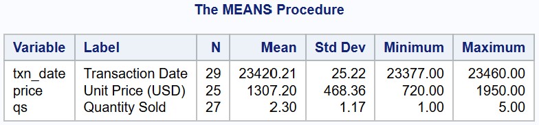
PROC MEANS DATA=sales_data MAXDEC=2;RUN;

Observe that PROC MEANS outputs summary statistics for the three quantitative variables: txn_date,[1] price, qs.
By default, PROC MEANS calculates the number of non-missing values, mean, the standard deviation, and the minimum and maximum values for each numeric variable. You can, however, also explicitly request specific summary statistics by including the following keywords in the PROC MEANS statement. Only the specified statistics will be calculated:
- MAX: Maximum value
- MIN: Minimum value
- MEAN: Mean value
- MEDIAN: Median
- MODE: Mode
- N: Number of non-missing values
- NMISS: Number of missing values
- RANGE: Range (maximum - minimum)
- STDDEV: Standard deviation
- SUM: Sum of values.
For example:
PROC MEANS DATA=sales_data NMISS N MEAN SUM;RUN;

If you run the PROC MEANS with no additional statements, it calculates summary statistics for all numeric variables across all groups. To specify which variables to analyze or to control the grouping, use the following statements after the PROC MEANS statement:
- BY <Variable-list>: Performs separate analyses for each unique combination of the values of the grouping variables. It is worth noting that the input data must first be sorted by the variables specified in the BY statement. Use PROC SORT to sort the data beforehand.
- CLASS <Variable-list>: Similar to the BY statement, CLASS also performs separate analyses for each unique combination of the values of the listed variables. However, the resulting table is more compact than that produced by BY, and, importantly, the input data does not need to be pre-sorted.
- VAR <Variable-list>: Specifies which numeric variables to be included in the analysis. If the VAR statement is omitted, PROC MEANS will analyze all numeric variables in the dataset.
For example:
DATA sales_data2;    SET sales_data;    txn_month = MONTH(txn_date);    sales_revenue = price * qs;RUN;
PROC MEANS DATA=sales_data2;    TITLE1 "Monthly Revenue Statistics";    TITLE2 "By Transaction Month (CLASS)";    CLASS txn_month;    VAR sales_revenue;RUN;
PROC SORT DATA=sales_data2;    BY txn_month;RUN;
PROC MEANS DATA=sales_data2;    TITLE2 "By Transaction Month (BY)";    BY txn_month;    VAR sales_revenue;RUN;

When calculating summary statistics, PROC MEANS excludes any missing values. This applies to both the numeric variables being analyzed and the grouping variables (specified using the BY or CLASS statement). If you want to include missing values as a valid grouping level, you should use the MISSING option in the PROC MEANS statement. For example, in the sales_data, there is a missing value for the sales_rep variable. Now, let's run the following two procedures and compare the results:
PROC MEANS DATA=sales_data2;    TITLE "Without MISSING Option";    CLASS rep;    VAR sales_revenue;RUN;
PROC MEANS DATA=sales_data2 MISSING;    TITLE "With MISSING Option";    CLASS rep;    VAR sales_revenue;RUN;

Observe that when the MISSING option is specified in the PROC MEANS, one more grouping level is added to represent the group of missing sales representatives, and calculations are performed for this group separately. This could be useful to see what's going on for the observations with the missing values.
The summary statistics calculated by PROC MEANS can be saved separately by adding the OUTPUT statement:
OUTPUT OUT = <Dataset-name> <Output-statistic = variable-name>;
Where:
- Dataset-name: Name of the dataset that will contain the results.
- Output-statistics = variable-names: Included statistics in the resulting dataset. Specify a statistic and its corresponding variable name. For the same summary statistic, you can list more than one variables. This will perform the same calculations for all the variables listed in the statement. Note that the order of the variables in the VAR and the OUTPUT statement must match in this case. If you want to have different summary statistics, add another OUTPUT statement in the procedure.
Additionally, you can add the NOPRINT option in the PROC MEANS statement, if your intention is just saving the calculated summary statistics in a separate dataset. For example:
PROC MEANS DATA=sales_data NOPRINT; CLASS rep; VAR price qs; OUTPUT OUT = sales_report MEAN(price qs) = price_by_rep qs_by_rep;RUN;

When working with quantitative variables, summarizing key metrics such as the average, total, minimum, and maximum values is a useful initial step for understanding overall trends. PROC MEANS in SAS provides a straightforward way to calculate these statistics across different categories.
The procedure begins with the two keywords PROC MEANS followed by optional parameters that control the analysis:
- MAXDEC=n: This option controls the maximum number of decimal places displayed in output. The value n specifies the desired number of decimal places. If MAXDEC is not explicitly set, the default value is 6.
- MISSING: Treats missing values as a valid group for summary calculations.
For example:
PROC MEANS DATA=sales_data MAXDEC=2;RUN;
Observe that PROC MEANS outputs summary statistics for the three quantitative variables: txn_date,[1] price, qs.
By default, PROC MEANS calculates the number of non-missing values, mean, the standard deviation, and the minimum and maximum values for each numeric variable. You can, however, also explicitly request specific summary statistics by including the following keywords in the PROC MEANS statement. Only the specified statistics will be calculated:
- MAX: Maximum value
- MIN: Minimum value
- MEAN: Mean value
- MEDIAN: Median
- MODE: Mode
- N: Number of non-missing values
- NMISS: Number of missing values
- RANGE: Range (maximum - minimum)
- STDDEV: Standard deviation
- SUM: Sum of values.
For example:
PROC MEANS DATA=sales_data NMISS N MEAN SUM;RUN;

If you run the PROC MEANS with no additional statements, it calculates summary statistics for all numeric variables across all groups. To specify which variables to analyze or to control the grouping, use the following statements after the PROC MEANS statement:
- BY <Variable-list>: Performs separate analyses for each unique combination of the values of the grouping variables. It is worth noting that the input data must first be sorted by the variables specified in the BY statement. Use PROC SORT to sort the data beforehand.
- CLASS <Variable-list>: Similar to the BY statement, CLASS also performs separate analyses for each unique combination of the values of the listed variables. However, the resulting table is more compact than that produced by BY, and, importantly, the input data does not need to be pre-sorted.
- VAR <Variable-list>: Specifies which numeric variables to be included in the analysis. If the VAR statement is omitted, PROC MEANS will analyze all numeric variables in the dataset.
For example:
DATA sales_data2;SET sales_data;txn_month = MONTH(txn_date);sales_revenue = price * qs;RUN;PROC MEANS DATA=sales_data2;TITLE1 "Monthly Revenue Statistics";TITLE2 "By Transaction Month (CLASS)";CLASS txn_month;VAR sales_revenue;RUN;PROC SORT DATA=sales_data2;BY txn_month;RUN;PROC MEANS DATA=sales_data2;TITLE2 "By Transaction Month (BY)";BY txn_month;VAR sales_revenue;RUN;

When calculating summary statistics, PROC MEANS excludes any missing values. This applies to both the numeric variables being analyzed and the grouping variables (specified using the BY or CLASS statement). If you want to include missing values as a valid grouping level, you should use the MISSING option in the PROC MEANS statement. For example, in the sales_data, there is a missing value for the sales_rep variable. Now, let's run the following two procedures and compare the results:
PROC MEANS DATA=sales_data2;TITLE "Without MISSING Option";CLASS rep;VAR sales_revenue;RUN;PROC MEANS DATA=sales_data2 MISSING;TITLE "With MISSING Option";CLASS rep;VAR sales_revenue;RUN;

Observe that when the MISSING option is specified in the PROC MEANS, one more grouping level is added to represent the group of missing sales representatives, and calculations are performed for this group separately. This could be useful to see what's going on for the observations with the missing values.
The summary statistics calculated by PROC MEANS can be saved separately by adding the OUTPUT statement:
OUTPUT OUT = <Dataset-name> <Output-statistic = variable-name>;
Where:
- Dataset-name: Name of the dataset that will contain the results.
- Output-statistics = variable-names: Included statistics in the resulting dataset. Specify a statistic and its corresponding variable name. For the same summary statistic, you can list more than one variables. This will perform the same calculations for all the variables listed in the statement. Note that the order of the variables in the VAR and the OUTPUT statement must match in this case. If you want to have different summary statistics, add another OUTPUT statement in the procedure.
Additionally, you can add the NOPRINT option in the PROC MEANS statement, if your intention is just saving the calculated summary statistics in a separate dataset. For example:
PROC MEANS DATA=sales_data NOPRINT;CLASS rep;VAR price qs;OUTPUT OUT = sales_report MEAN(price qs) = price_by_rep qs_by_rep;RUN;

Creating Frequency Distribution Tables Using PROC FREQ
A frequency distribution table is a way to organize and summarize data by showing how often each value (or range of values) appear in a dataset. It tells you the count of data points for each category, helping to identify patterns, trends, and distributions within the data.
In SAS, you can create a frequency distribution table using PROC FREQ. For example:
PROC FREQ DATA=sales_data; TABLES prod;RUN;

To combine more than one variables for the counts, you can simply list the variables in the TABLES statement, separating each variable with an asterisk. For example:
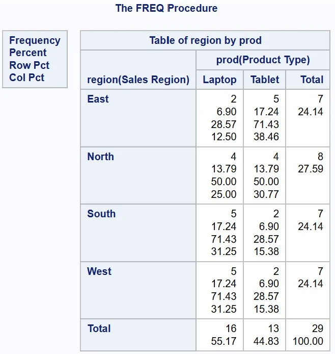
PROC FREQ DATA=sales_data; TABLES region * prod;RUN;
Options, if any, should appear after the variables and a slash in the TABLES statement. They control the output of the PROC FREQ results.
- LIST: Prints frequency distribution tables in a list format, not grid.
- MISSPRINT: Counts missing values in frequencies, but not in percentages.
- MISSING: Counts missing values in both frequencies and percentages.
- NOCOL: Do not print column percentages.
- NOROW: Do not print row percentages.
- NOPERCENT: Do not print percentages.
- OUT = <data-set-name>: Save the results as a new dataset.
For example:
PROC FREQ DATA=sales_data; TABLES region * prod / MISSPRINT NOCOL;RUN;

A frequency distribution table is a way to organize and summarize data by showing how often each value (or range of values) appear in a dataset. It tells you the count of data points for each category, helping to identify patterns, trends, and distributions within the data.
In SAS, you can create a frequency distribution table using PROC FREQ. For example:
PROC FREQ DATA=sales_data;TABLES prod;RUN;

To combine more than one variables for the counts, you can simply list the variables in the TABLES statement, separating each variable with an asterisk. For example:
PROC FREQ DATA=sales_data;TABLES region * prod;RUN;

Options, if any, should appear after the variables and a slash in the TABLES statement. They control the output of the PROC FREQ results.
- LIST: Prints frequency distribution tables in a list format, not grid.
- MISSPRINT: Counts missing values in frequencies, but not in percentages.
- MISSING: Counts missing values in both frequencies and percentages.
- NOCOL: Do not print column percentages.
- NOROW: Do not print row percentages.
- NOPERCENT: Do not print percentages.
- OUT = <data-set-name>: Save the results as a new dataset.
For example:
PROC FREQ DATA=sales_data;TABLES region * prod / MISSPRINT NOCOL;RUN;

Aside: Reshaping Data from Long to Wide Using PROC TRANSPOSE
Suppose you have the following data about monthly sales for different regions and product categories. The data includes sales region, product, sales month, and sales amount:
North Electronics Jan-2023 10000North Furniture Jan-2023 7000North Electronics Feb-2023 12000North Furniture Feb-2023 8000South Electronics Jan-2023 15000South Furniture Jan-2023 5000South Electronics Feb-2023 14000South Furniture Feb-2023 6000
In this scenario, the primary variable of interest is the sales amount for each combination of sales region and products. Specifically, you want to compare the sales amount for January and February, so that you can identify regional and product-specific sales trends.
However, the current dataset presents sales data for a specific product across regions and month in a distributed manner. For instance, the sales amount for "Electronics" in January 2023 is located at the first observation, while that for Feb-2023 is in the third). This arrangement, where relevant data points are spread across rows instead of being aligned horizontally, makes it difficult to contrast sales performance across the three dimensions (i.e., region, product category, and sales month).
To reshape this dataset for a side-by-side comparisons, use PROC TRANSPOSE. This procedure transforms data by switching rows and columns. In most cases, to convert observations into variables, you can use the following statements:
PROC TRANSPOSE DATA=<Current-dataset> OUT=<Transposed-dataset>; BY <BY-variable-list>; ID <ID-variable-list>; VAR <VAR-variable-list>;RUN;
Where:
- Current-dataset: The name of the dataset you want to transpose. If omitted, the most recently created SAS dataset will be used.
- Transposed-dataset: The name of the transposed output dataset. If omitted, it defaults to work.outdata.
- BY-variable-list: Specifies the variables that define the grouping of the data. These variables must be present in an order and are used to keep rows grouped together during transposition.
- ID-variable-list: Specifies the variables that will become the column names in the transposed dataset.
- VAR-variable-list: Variables which will be transposed into the values for each observation in the output dataset.
For example:
DATA raw_sales;    INPUT region $ product :$11. sales_month $ sales_amount;    DATALINES;North Electronics Jan-2023 10000 North Furniture   Jan-2023 7000North Electronics Feb-2023 12000North Furniture   Feb-2023 8000South Electronics Jan-2023 15000South Furniture   Jan-2023 5000South Electronics Feb-2023 14000South Furniture   Feb-2023 6000;RUN;
/* Sort raw_sales by region and product */PROC SORT DATA=raw_sales;    BY region product;RUN;
/* Transpose data for direct comparisons */PROC TRANSPOSE DATA=raw_sales OUT=transposed_sales;    BY region product;    ID sales_month;    VAR sales_amount;RUN;
As with BY statements in other procedures, the BY statement of PROC TRANSPOSE requires the input data to be pre-sorted by the BY variables, which can be achieved using PROC SORT. Then, in the PROC TRANSPOSE, the BY statement groups the data by region and product. The ID statement, using sales_month, specifies that the values in this variable (e.g., "Jan-2023" and "Feb-2023") will become new column names in the transposed dataset. Lastly, the VAR statement, using sales_amount, indicates that the sales_amount variable will be transposed into corresponding columns based on the sales_month values.

Now in this format, data for different months is arranged horizontally, making it easy to perform direct side-by-side comparisons. For example, you can quickly see that electronic sales in the South region decreased in February, while sales of other products in both the North and South region increased during the same period. This layout improves the interpretability and efficiency of sales reporting by providing a clear, comparative view of the key metrics.
Suppose you have the following data about monthly sales for different regions and product categories. The data includes sales region, product, sales month, and sales amount:
North Electronics Jan-2023 10000North Furniture Jan-2023 7000North Electronics Feb-2023 12000North Furniture Feb-2023 8000South Electronics Jan-2023 15000South Furniture Jan-2023 5000South Electronics Feb-2023 14000South Furniture Feb-2023 6000
In this scenario, the primary variable of interest is the sales amount for each combination of sales region and products. Specifically, you want to compare the sales amount for January and February, so that you can identify regional and product-specific sales trends.
However, the current dataset presents sales data for a specific product across regions and month in a distributed manner. For instance, the sales amount for "Electronics" in January 2023 is located at the first observation, while that for Feb-2023 is in the third). This arrangement, where relevant data points are spread across rows instead of being aligned horizontally, makes it difficult to contrast sales performance across the three dimensions (i.e., region, product category, and sales month).
To reshape this dataset for a side-by-side comparisons, use PROC TRANSPOSE. This procedure transforms data by switching rows and columns. In most cases, to convert observations into variables, you can use the following statements:
PROC TRANSPOSE DATA=<Current-dataset> OUT=<Transposed-dataset>;BY <BY-variable-list>;ID <ID-variable-list>;VAR <VAR-variable-list>;RUN;
Where:
- Current-dataset: The name of the dataset you want to transpose. If omitted, the most recently created SAS dataset will be used.
- Transposed-dataset: The name of the transposed output dataset. If omitted, it defaults to work.outdata.
- BY-variable-list: Specifies the variables that define the grouping of the data. These variables must be present in an order and are used to keep rows grouped together during transposition.
- ID-variable-list: Specifies the variables that will become the column names in the transposed dataset.
- VAR-variable-list: Variables which will be transposed into the values for each observation in the output dataset.
For example:
DATA raw_sales;INPUT region $ product :$11. sales_month $ sales_amount;DATALINES;North Electronics Jan-2023 10000North Furniture Jan-2023 7000North Electronics Feb-2023 12000North Furniture Feb-2023 8000South Electronics Jan-2023 15000South Furniture Jan-2023 5000South Electronics Feb-2023 14000South Furniture Feb-2023 6000;RUN;/* Sort raw_sales by region and product */PROC SORT DATA=raw_sales;BY region product;RUN;/* Transpose data for direct comparisons */PROC TRANSPOSE DATA=raw_sales OUT=transposed_sales;BY region product;ID sales_month;VAR sales_amount;RUN;
As with BY statements in other procedures, the BY statement of PROC TRANSPOSE requires the input data to be pre-sorted by the BY variables, which can be achieved using PROC SORT. Then, in the PROC TRANSPOSE, the BY statement groups the data by region and product. The ID statement, using sales_month, specifies that the values in this variable (e.g., "Jan-2023" and "Feb-2023") will become new column names in the transposed dataset. Lastly, the VAR statement, using sales_amount, indicates that the sales_amount variable will be transposed into corresponding columns based on the sales_month values.

Now in this format, data for different months is arranged horizontally, making it easy to perform direct side-by-side comparisons. For example, you can quickly see that electronic sales in the South region decreased in February, while sales of other products in both the North and South region increased during the same period. This layout improves the interpretability and efficiency of sales reporting by providing a clear, comparative view of the key metrics.
Producing Tabular Reports with PROC TABULATE
PROC TABULATE is a SAS procedure that can create a professional-grade reports. In fact, every summary statistic that the TABULATE procedure computes can also be produced by other procedures, such as MEAN or FREQ. However, PROC TABULATE can create a well-structured, visually appealing reports with neatly formatted tables and customizable layouts.
The PROC TABULATE has the following general syntax:
PROC TABULATE DATA=<Input-dataset> [MISSING]; CLASS <Grouping-variable-list>; TABLE [[<page-dimension>,] <row-dimension>,] <column-dimension>;RUN;
Where:
- MISSING: By default, PROC TABULATE excludes observations with missing values for variables listed in the CLASS statement. If you want to include those observations, you should use the MISSING option in the PROC TABULATE statement.
- CLASS: Specifies the list of grouping variables.
- TABLE: Defines the output table structure. Up to three variables can be specified: One for columns, two for rows and columns, and three for page, row, and column dimensions. Each dimension should be separated by a comma.
For example:
PROC TABULATE DATA=sales_data; TITLE1 "Frequency Table"; TITLE2 "By Product"; FOOTNOTE "TABLE prod;"; CLASS prod; TABLE prod;RUN;

If you have two variables in the TABLE statement, the variables will be used as row and column dimensions. Please note that all grouping variables that you will use in the TABLE statement must also be presented in the CLASS statement:
PROC TABULATE DATA=sales_data; TITLE2 "By Sales Representative and Product"; FOOTNOTE "TABLE rep prod;"; CLASS rep prod; TABLE rep, prod;RUN;

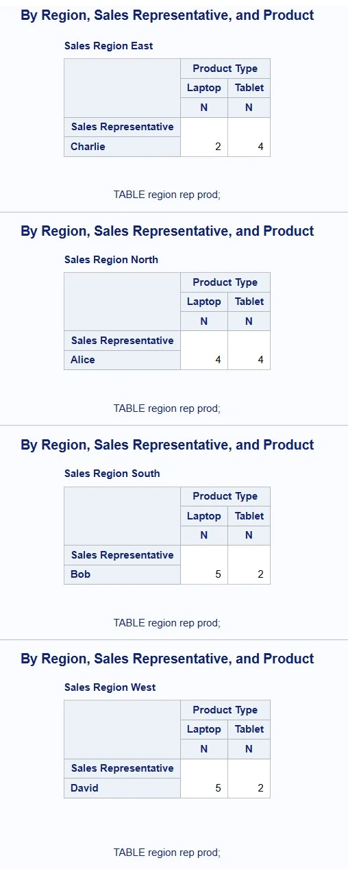
If you specify three variables in the TABLE statement, the variables will be used to specify page, row, and column dimensions, accordingly. For example:
PROC TABULATE DATA=sales_data; TITLE2 "By Region, Sales Representative, and Product"; FOOTNOTE "TABLE region rep prod;"; CLASS region rep prod; TABLE region, rep, prod;RUN;
PROC TABULATE is a SAS procedure that can create a professional-grade reports. In fact, every summary statistic that the TABULATE procedure computes can also be produced by other procedures, such as MEAN or FREQ. However, PROC TABULATE can create a well-structured, visually appealing reports with neatly formatted tables and customizable layouts.
The PROC TABULATE has the following general syntax:
PROC TABULATE DATA=<Input-dataset> [MISSING];CLASS <Grouping-variable-list>;TABLE [[<page-dimension>,] <row-dimension>,] <column-dimension>;RUN;
Where:
- MISSING: By default, PROC TABULATE excludes observations with missing values for variables listed in the CLASS statement. If you want to include those observations, you should use the MISSING option in the PROC TABULATE statement.
- CLASS: Specifies the list of grouping variables.
- TABLE: Defines the output table structure. Up to three variables can be specified: One for columns, two for rows and columns, and three for page, row, and column dimensions. Each dimension should be separated by a comma.
For example:
PROC TABULATE DATA=sales_data;TITLE1 "Frequency Table";TITLE2 "By Product";FOOTNOTE "TABLE prod;";CLASS prod;TABLE prod;RUN;

If you have two variables in the TABLE statement, the variables will be used as row and column dimensions. Please note that all grouping variables that you will use in the TABLE statement must also be presented in the CLASS statement:
PROC TABULATE DATA=sales_data;TITLE2 "By Sales Representative and Product";FOOTNOTE "TABLE rep prod;";CLASS rep prod;TABLE rep, prod;RUN;

If you specify three variables in the TABLE statement, the variables will be used to specify page, row, and column dimensions, accordingly. For example:
PROC TABULATE DATA=sales_data;TITLE2 "By Region, Sales Representative, and Product";FOOTNOTE "TABLE region rep prod;";CLASS region rep prod;TABLE region, rep, prod;RUN;

PROC TABULATE with Summary Statistics
With no other statements are specified, PROC TABULATE creates frequency tables. These tables show the count of observations for each level of the variables listed in the CLASS statement. However, you can add the VAR statement with quantitative variables to include some summary statistics instead of the basic counts in your output. Here is the general syntax of the PROC TABULATE with the VAR statement:
PROC TABULATE DATA=<Input-dataset> [MISSING]; VAR <Analysis-variable-list>; CLASS <Grouping-variable-list>; TABLE [[<page-dimension>,] <row-dimension>,] <column-dimension>;RUN;
You can include both a CLASS statement and a VAR statement, or just one of them. However, all variables listed in the TABLE statement must also be present at least one of the CLASS or VAR statement.
If you just specify the VAR variable without any specific summary statistic request, then will calculate the SUM by default. For example:
PROC TABULATE DATA=sales_data; VAR qs; CLASS prod; TABLE prod, qs;RUN;

Instead of the default sum, you can also explicitly request specific calculations. Here is the list of available options:
- MIN: Minimum value
- MAX: Maximum value
- MEAN: Arithmetic mean
- MEDIAN: Median
- MODE: Mode
- N: Number of non-missing values
- NMISS: Number of missing values
- PCTN: Percentage of observations for each CLASS group
- PCTSUM: Percentage of total represented by each CLASS group
- STDDEV: Standard deviation
- SUM: Sum
- ALL: Adds a row, column, or page total
Within each dimension (page, row, or column), you can add these keyword after the associated variable and an asterisk (*) in the TABLE statement (e.g., qs*MIN). You can also list more than one calculations, with each separated by a space. For example:
PROC TABULATE DATA=sales_data; VAR qs; CLASS prod; TABLE prod, qs*MIN qs*MAX qs*SUM;RUN;

In PROC TABULATE, crossing variables creates a table where the values of one variable form the rows, and the values of another variable form the columns. This allows you to see the combinations of values between the two variables and calculate statistics for each combination. For example:
PROC TABULATE DATA=sales_data; VAR qs; CLASS prod region; TABLE prod * region, qs*MIN qs*MAX qs*SUM;RUN;

In this example, two dimensions are specified in the TABLE statement: row and column. The two dimensions are separated by a comma in the statement. Within the row dimension, the product type and sales region are crossed, so that within a product type, observations are sub-grouped by the region.
Observe that the columns represent minimum, maximum, and summation for the same variable (qs). So, in this case, the TABLE statement can be revised as follows:
PROC TABULATE DATA=sales_data; VAR qs; CLASS prod region; TABLE prod * region, qs * (MIN MAX SUM);RUN;
You can think of the asterisk and parentheses for the column dimension in this example as "distribution law" of the mathematical formula--the values for qs are "distributed" across the statistics. Here is the result:

To sum up, the TABLE statement in PROC TABULATE defines the structure of your table. You list the variables specified in the CLASS and VAR statements; CLASS variables define the rows, columns, and pages (dimensions), while VAR variables are the data being summarized.
The TABLE statement can have up to three dimensions, separated by commas. If there is only one dimension, it defines the column dimension. If two dimensions are specified, your output will be grouped by rows and columns. If all three dimensions are specified, each will represent page, row, and columns, respectively.
Within each dimension, an asterisk creates all possible combinations of the variables. For example, region * product within the row dimension would creates cells for each region-product pairing, with product values nested inside their respective regions. The combination can also include a specific keyword for a desired output. For instance, MEAN * product * revenue means calculate the average for each product.
On the other hand, if variables and/or metrics are separated by blank spaces within a dimension, it concatenates them, adding one more levels for the dimension. With all this in mind, let's create complex tables for practice!
PROC TABULATE DATA=sales_data;    TITLE "Table 1";    VAR price qs;    CLASS region prod rep;    TABLE region * (prod * (rep * (MEAN*price SUM*qs)));RUN;
PROC TABULATE DATA=sales_data;    TITLE "Table 2";    VAR price qs;    CLASS region prod rep;    TABLE region prod rep * (MEAN*price SUM*qs);RUN;
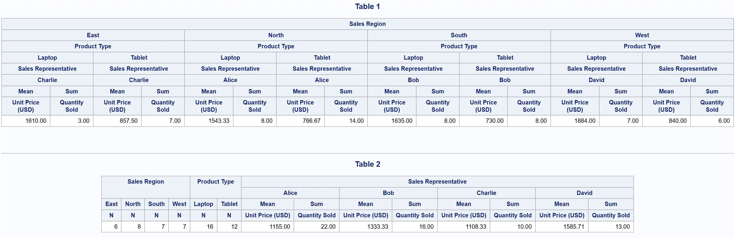
The TABLE statement in the first PROC TABULATE has a single dimension. So all metrics and variables will be used to define columns. At its lowest level, the average price (MEAN*price) and total quantity sold (SUM*qs) are nested within each sales representative (rep). The sales representatives are then nested within each product (prod), and the products are nested within each sales region (region).
Similarly, in the second PROC TABULATE, we only have the column dimension. The table columns are defined by the concatenation of region, products, and sales representatives, with the average price and total quantity sold is nested within the sales representatives.
You can practice for row and page dimensions with the same manner. A good strategy for building TABLE statement is to begin with the column dimension. After verifying the column structure, add the row dimension. If a page dimension is required, include it last. Notice that the order of dimensions in the TABLE statement is page, row, and column. So, to avoid scrambling your table when you add dimensions, insert the row specifications in front of the column dimension. Similarly, after checking the column and row dimensions, include the page dimension in front of the row dimension. This makes it easier to incrementally develop and test your table structure.
With no other statements are specified, PROC TABULATE creates frequency tables. These tables show the count of observations for each level of the variables listed in the CLASS statement. However, you can add the VAR statement with quantitative variables to include some summary statistics instead of the basic counts in your output. Here is the general syntax of the PROC TABULATE with the VAR statement:
PROC TABULATE DATA=<Input-dataset> [MISSING];VAR <Analysis-variable-list>;CLASS <Grouping-variable-list>;TABLE [[<page-dimension>,] <row-dimension>,] <column-dimension>;RUN;
You can include both a CLASS statement and a VAR statement, or just one of them. However, all variables listed in the TABLE statement must also be present at least one of the CLASS or VAR statement.
If you just specify the VAR variable without any specific summary statistic request, then will calculate the SUM by default. For example:
PROC TABULATE DATA=sales_data;VAR qs;CLASS prod;TABLE prod, qs;RUN;

Instead of the default sum, you can also explicitly request specific calculations. Here is the list of available options:
- MIN: Minimum value
- MAX: Maximum value
- MEAN: Arithmetic mean
- MEDIAN: Median
- MODE: Mode
- N: Number of non-missing values
- NMISS: Number of missing values
- PCTN: Percentage of observations for each CLASS group
- PCTSUM: Percentage of total represented by each CLASS group
- STDDEV: Standard deviation
- SUM: Sum
- ALL: Adds a row, column, or page total
Within each dimension (page, row, or column), you can add these keyword after the associated variable and an asterisk (*) in the TABLE statement (e.g., qs*MIN). You can also list more than one calculations, with each separated by a space. For example:
PROC TABULATE DATA=sales_data;VAR qs;CLASS prod;TABLE prod, qs*MIN qs*MAX qs*SUM;RUN;

In PROC TABULATE, crossing variables creates a table where the values of one variable form the rows, and the values of another variable form the columns. This allows you to see the combinations of values between the two variables and calculate statistics for each combination. For example:
PROC TABULATE DATA=sales_data;VAR qs;CLASS prod region;TABLE prod * region, qs*MIN qs*MAX qs*SUM;RUN;

In this example, two dimensions are specified in the TABLE statement: row and column. The two dimensions are separated by a comma in the statement. Within the row dimension, the product type and sales region are crossed, so that within a product type, observations are sub-grouped by the region.
Observe that the columns represent minimum, maximum, and summation for the same variable (qs). So, in this case, the TABLE statement can be revised as follows:
PROC TABULATE DATA=sales_data;VAR qs;CLASS prod region;TABLE prod * region, qs * (MIN MAX SUM);RUN;
You can think of the asterisk and parentheses for the column dimension in this example as "distribution law" of the mathematical formula--the values for qs are "distributed" across the statistics. Here is the result:

To sum up, the TABLE statement in PROC TABULATE defines the structure of your table. You list the variables specified in the CLASS and VAR statements; CLASS variables define the rows, columns, and pages (dimensions), while VAR variables are the data being summarized.
The TABLE statement can have up to three dimensions, separated by commas. If there is only one dimension, it defines the column dimension. If two dimensions are specified, your output will be grouped by rows and columns. If all three dimensions are specified, each will represent page, row, and columns, respectively.
Within each dimension, an asterisk creates all possible combinations of the variables. For example, region * product within the row dimension would creates cells for each region-product pairing, with product values nested inside their respective regions. The combination can also include a specific keyword for a desired output. For instance, MEAN * product * revenue means calculate the average for each product.
On the other hand, if variables and/or metrics are separated by blank spaces within a dimension, it concatenates them, adding one more levels for the dimension. With all this in mind, let's create complex tables for practice!
PROC TABULATE DATA=sales_data;TITLE "Table 1";VAR price qs;CLASS region prod rep;TABLE region * (prod * (rep * (MEAN*price SUM*qs)));RUN;PROC TABULATE DATA=sales_data;TITLE "Table 2";VAR price qs;CLASS region prod rep;TABLE region prod rep * (MEAN*price SUM*qs);RUN;

The TABLE statement in the first PROC TABULATE has a single dimension. So all metrics and variables will be used to define columns. At its lowest level, the average price (MEAN*price) and total quantity sold (SUM*qs) are nested within each sales representative (rep). The sales representatives are then nested within each product (prod), and the products are nested within each sales region (region).
Similarly, in the second PROC TABULATE, we only have the column dimension. The table columns are defined by the concatenation of region, products, and sales representatives, with the average price and total quantity sold is nested within the sales representatives.
You can practice for row and page dimensions with the same manner. A good strategy for building TABLE statement is to begin with the column dimension. After verifying the column structure, add the row dimension. If a page dimension is required, include it last. Notice that the order of dimensions in the TABLE statement is page, row, and column. So, to avoid scrambling your table when you add dimensions, insert the row specifications in front of the column dimension. Similarly, after checking the column and row dimensions, include the page dimension in front of the row dimension. This makes it easier to incrementally develop and test your table structure.
Styling PROC TABULATE Outputs
Formatting Data Cells
In the PROC TABULATE statement, you can add the FORMAT= option to specify a specific data format for all output table cells. For example:
PROC TABULATE DATA=sales_data FORMAT=DOLLAR9.2; VAR price; CLASS prod; TABLE MEAN * price, prod;RUN;

When a PROC TABULATE table contains different data types, applying distinct formats to each type would be desirable. However, the FORMAT= option in the PROC TABULATE statement applies a single format to all cells, making this direct approach unsuitable.
To apply a format to an individual variable, cross it with the variable name like this:
<Variable-name> * FORMAT = formatw.d
Then you can insert this rather convoluted construction in your TABLE statement. For example:
PROC TABULATE DATA=sales_data; VAR price qs; CLASS prod region; TABLE region, MEAN * prod * (price * FORMAT=DOLLAR9.2 qs * FORMAT=COMMA8.0);RUN;

In the PROC TABULATE statement, you can add the FORMAT= option to specify a specific data format for all output table cells. For example:
PROC TABULATE DATA=sales_data FORMAT=DOLLAR9.2;VAR price;CLASS prod;TABLE MEAN * price, prod;RUN;

When a PROC TABULATE table contains different data types, applying distinct formats to each type would be desirable. However, the FORMAT= option in the PROC TABULATE statement applies a single format to all cells, making this direct approach unsuitable.
To apply a format to an individual variable, cross it with the variable name like this:
<Variable-name> * FORMAT = formatw.d
Then you can insert this rather convoluted construction in your TABLE statement. For example:
PROC TABULATE DATA=sales_data;VAR price qs;CLASS prod region;TABLE region, MEAN * prod * (price * FORMAT=DOLLAR9.2 qs * FORMAT=COMMA8.0);RUN;

Customizing Empty Cells
In general, PROC TABULATE leaves the upper-left corner of the report entirely empty. This empty box left black as it falls outside the intersection of row and column variables. You can, however, specify some text that will populate the corner using the BOX= option in the TABLE statement. For example:
PROC TABULATE DATA=sales_data FORMAT=DOLLAR9.2; VAR price; CLASS prod; TABLE MEAN * price, prod / BOX="Average Price by Product";RUN;

The MISSTEXT= option, on the other hand, specifies a value for SAS to print in the data cells where there is no value present. For example:
PROC TABULATE DATA=sales_data MISSING;
    CLASS rep prod;
    VAR price qs;
    TABLE rep, prod*(price qs)*MEAN / MISSTEXT="NA";
RUN;
Remember that the raw dataset has a missing value for the sales representative variable (rep), and the PROC TABULATE example shown above uses the MISSING option to ensure that missing value is included in the table. Specifically, any cell at the intersection of a missing rep value and a prod value will initially be empty.
The MISSTEXT="NA" option, included in the TABLE statement, then populates these empty intersection cells with "NA." This will populate the empty cells with the text "NA," making the table easier to interpret. Here is the result.

In general, PROC TABULATE leaves the upper-left corner of the report entirely empty. This empty box left black as it falls outside the intersection of row and column variables. You can, however, specify some text that will populate the corner using the BOX= option in the TABLE statement. For example:
PROC TABULATE DATA=sales_data FORMAT=DOLLAR9.2;VAR price;CLASS prod;TABLE MEAN * price, prod / BOX="Average Price by Product";RUN;

The MISSTEXT= option, on the other hand, specifies a value for SAS to print in the data cells where there is no value present. For example:
PROC TABULATE DATA=sales_data MISSING; CLASS rep prod; VAR price qs; TABLE rep, prod*(price qs)*MEAN / MISSTEXT="NA"; RUN;
Remember that the raw dataset has a missing value for the sales representative variable (rep), and the PROC TABULATE example shown above uses the MISSING option to ensure that missing value is included in the table. Specifically, any cell at the intersection of a missing rep value and a prod value will initially be empty.
The MISSTEXT="NA" option, included in the TABLE statement, then populates these empty intersection cells with "NA." This will populate the empty cells with the text "NA," making the table easier to interpret. Here is the result.


0 Comments