In the everyday practice of SAS programming, we casually say that executing a PROC step creates its output, but that's not quite true. Technically, what a PROC step creates is just the data itself, not the formatted result we can see. Then, a separate program called Output Delivery Systems (ODS) takes the data values and sends them to the destination. You can think of the ODS as a post office; just as postal workers deliver parcels to their designated recipients through its appropriate delivery methods, the ODS receives data from a procedure and distributes them to their destination through templates.
When you working in the ODS environment, a destination refers to the file format to which ODS routes its output, which can be categorized into either a SAS formatted destinations or a third-party formatted destinations. The SAS formatted destinations generate an output file that is controlled and interpreted by SAS, such as SAS data set, ODS document, or a text output. On the other hand, third-party destinations produce an output like HTML, PDF, or RTF, which is the most common scenario when using ODS statements.
The table below outlines the ODS destinations and the resulting formatted outputs:
| Category | Destinations | Results |
| SAS Formatted | DOCUMENT | ODS document. |
| LISTING | Text output. Default destination when you run a SAS program in batch or on operating system other than Windows or UNIX. To generate a third-party formatted file in these environments, you should use an ODS statement. | |
| OUTPUT | SAS data set in the "Output" tab. | |
| Third-party Formatted | HTML | HTML file for web page. Default destination on Microsoft Windows and UNIX (starting with SAS 9.3). |
| MARKUP | Any output format that is defined tagsets, including XML, EXCELXP, LaTeX, CSV, etc. | |
| PRINTER | Printable output in one of three different formats: PCL, PDF, or PS (PostScript). | |
| RTF | Output written in Rich Text Format for use with word processor. |
In ODS, a table template acts like blueprints for your data's presentation. They define how your data will be structured, such as the arrangement of column headings, variable order, and overall layout. When ODS receives data from a procedure, it combines it with the chosen table template. This combined entity, containing both data and its formatting instructions, is called an output object.
This output object is then further elaborated by a style template, which defines the presentational aspects, such as background color or font size, for the entire SAS output. To see the overall list of available styles, please submit the following PROC TEMPLATE statements:
PROC TEMPLATE;LIST STYLES;RUN;
Tracing and Selecting Output Objects
Executing a PROC step basically creates a single set of data, which can be paired with a single table template to generate an output object. This output object has an unique name that can be traced and selected. For example:
DATA HeightWeight;INFILE '/home/u63368964/source/height-weight-v2.txt' DLM=',' DSD;INPUT Name :$15. Age Sex $ Weight Height;RUN;ODS TRACE ON;PROC MEANS DATA=HeightWeight;RUN;ODS TRACE OFF;
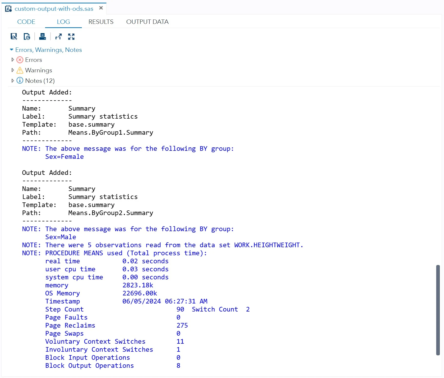
In the SAS program above, the global statement ODS TRACE ON prints output object in your SAS log. Then, after the RUN statement is submitted, ODS TRACE OFF turns off the trace.
If your procedure includes a BY statement, SAS creates a separate data set (and consequently, a separate output object) for each BY group. Each output object of a BY group has a unique name so that it can be traced and selected.
PROC SORT DATA=HeightWeight;BY Sex;RUN;ODS TRACE ON;PROC MEANS DATA=HeightWeight;BY Sex;RUN;ODS TRACE OFF;
Once you have identified the names of the output objects, you can select the ones by an ODS SELECT statement. The general form of an ODS SELECT statement is as follows:
<The PROC step with the output objects you want to select>ODS SELECT output-object-list;RUN;
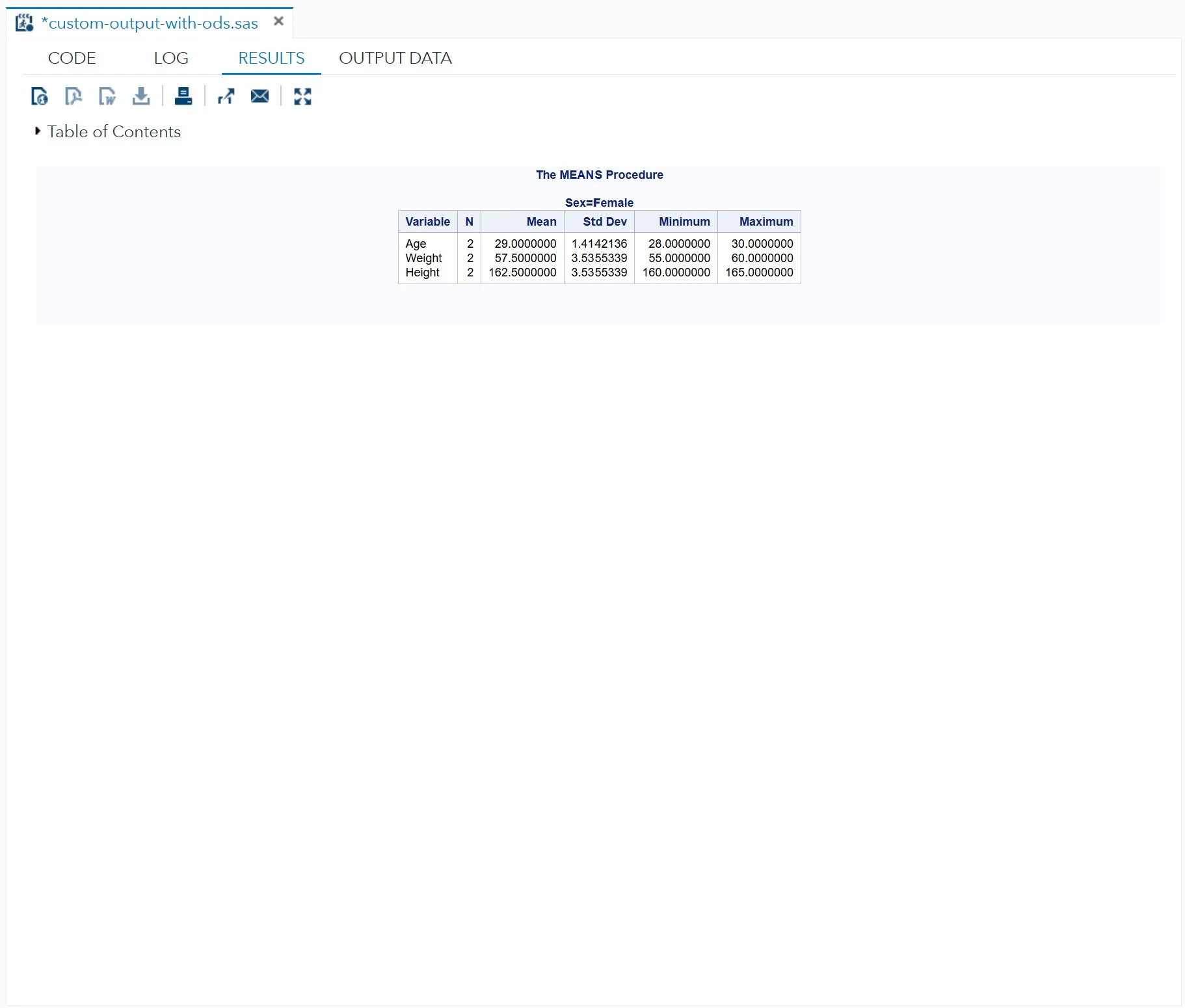
For example, the following program runs PROC MEANS again using the HeightWeight data set, and an ODS SELECT statement to select just the first output object: Means.ByGroup1.Summary. Consequently, only the first BY group is included in the result.
PROC MEANS DATA=HeightWeight;BY Sex;ODS SELECT Means.ByGroup1.Summary;RUN;
Alternatively, you can use an ODS EXCLUDE statement to exclude any listed output objects. Its general form is the same as that of ODS SELECT statement.
Creating HTML Outputs
The ODS HTML statement send the ODS output objects combined with the style template specification to the HTML destination files, which are ready to be posted on web pages. The general form of the statement is:
/* BODY= is synonymous with FILE= */ODS HTML FILE='path/to/file.html' options;
If you are working on the SAS Studio, the destination file path for the FILE= option always begins with '/home/your-user-name/'. You can find your user name at the bottom right corner on your browser. This option specifies location and name of the file which contains PROC results. Other options include:
- CONTENT = 'path/to/content/file.html': Creates a table of contents with links to the body file.
- PAGE = 'path/to/page/file.html': Creates a table of contents with links by page number.
- FRAME = 'path/to/frame/file.html': Creates a frame that allows you to view the body file and the contents or the page file at the same time. If you do not want either the contents or the page file, then you don't need to create a frame file.
- STYLE = style-name: Specifies a style template. The default setting is STYLE=HTMLBLUE.
ODS statements are global, and do not belong to either DATA steps or PROC steps. However, putting them in a wrong place could result in capturing the desired output. A good place to put the ODS HTML statement is just before the step (or steps) whose output you intend to capture. Then additionally, you can also include some text explanations to your ODS output, using the ODS TEXT= statement. Lastly, you should close the HTML destination using:
ODS HTML CLOSE;
For example:
ODS HTML STYLE=OCEANFILE='/home/u63368964/sasuser.v94/height-weight-body.html'FRAME='/home/u63368964/sasuser.v94/height-weight-frame.html'CONTENTS='/home/u63368964/sasuser.v94/height-weight-contents.html';PROC MEANS DATA=HeightWeight; TITLE "Height and Weight by Sex"; BY Sex; RUN;ODS TEXT='<div align="center">This is text after PROC MEANS output.</div>';ODS HTML CLOSE;
Creating RTF and PDF Outputs
Rich Text Format (RTF) is a file format designed to store formatted text and graphics. When you create an RTF output, you can further edit the texts and images of the file through word processor. The general form of the ODS statement to open RTF files is:
ODS RTF FILE='path/to/file.rtf' options;
Unlike HTML, the ODS RTF creates a single file that contains the output. Here are some commonly employed options for the destination:
- BODYTITLE: Puts title and footnotes in the main part of the RTF document instead of in Word headers or footers.
- COLUMNS = n: Requests columnar output where n is the number of columns.
- SASDATE: By default, the date and time that appear at the top of RTF output indicate when the file was last opened or printed in Word. This option tells SAS to use the date and time when the current SAS session or job started running.
- STARTPAGE = value: Controls page breaks. The default value, YES, inserts a page break between procedures. A value of NO turns off page breaks. A value of NOW inserts a page break at that point.
- STYLE = style-name: Specifies a style template. The default is RTF.
To close the RTF file, put this statement after the step (or steps) whose output you wish to capture, and following a RUN statement:
ODS RTF CLOSE;
For example:
ODS RTF FILE='/home/u63368964/sasuser.v94/height-weight.rtf' BODYTITLE STARTPAGE=NO;
ODS NOPROCTITLE;
PROC MEANS DATA=HeightWeight;
    TITLE 'Height and Weight by Sex';
    CLASS Sex;
RUN;

PROC PRINT DATA=HeightWeight;
RUN;

ODS RTF CLOSE;
Creating a PDF output is similar to creating an RTF output. Just as RTF destination, the PDF destination produces a single PDF file. The general form of the ODS statement is:
ODS PDF FILE='path/to/file.rtf' options;
The options available for the PDF destination include:
- COLUMNS = n: Requests columnar output where n is the number of columns.
- STARTPAGE = value: Controls page breaks. The default value, YES, inserts a break between procedures. A value of NO turns off breaks. A value of NOW inserts a break at that point.
- STYLE = style-name: Specifies a style template. The default is PRINTER.
Here is the ODS statement which closes the PDF file. Put this statement after the step (or steps) whose output you wish to capture, and following a RUN statement:
ODS PDF CLOSE;
ODS Graphics
ODS Graphics is an extension of the Output Delivery System, designed to create files with data visualizations using SAS. It uses the same destinations and styles as ODS tabular outputs, but instead of tables, ODS Graphics creates charts and graphs.
Since SAS 9.3, ODS Graphics is enabled by defaulted within the SAS windowing environment for both Microsoft Windows and UNIX. However, it's disabled by default when running in batch mode or other environments. To activate ODS Graphics manually, include the following statement at the beginning of your program, before any statistical procedures:
ODS GRAPHICS ON;
ODS Graphics persists only for the duration of your SAS session. So, in a typically situation, you do not need to turn it off manually. However, if you need to disable it for performance reasons or to exclude graphs from your output, use this statement:
ODS GRAPHICS OFF;
To specify properties for your images, use the ODS GRAPHICS statement with this general form:
ODS GRAPHICS / options;
Where available options are:
- HEIGHT = n: Specifies image height in CM, IN, MM, PT, or PX.
- WIDTH = n: Specifies image height in CM, IN, MM, PT, or PX.
- IMAGENAME = 'filename': Specifies the base image file name. It defaults to the name of its ODS output object.
- OUTPUTFMT = file-type: Specifies the graph format. Possible values include BMP, GIF, JPEG, PDF, PNG, PS, SVG, TIFF, and many others.
- RESET: Reset all options to their defaults.
Note that specifying only the width or height in ODS Graphics causes SAS to adjust the other dimension to maintain a default aspect ratio of 4:3. Typical choice for the graph size is 640 pixels wide by 480 pixels high.
Saving Graphical Output
To save a graphical output, you use an ODS destination statement with this general form:
ODS destination-name options;
Where:
- destination-name: Your ODS destination such as HTML, LISTING, PDF, or RTF.
- Options:
- FILE = 'path/filename': Specifies a path and file name for saving output images from the PDF and RTF destinations. Images will be saved in a single file along with tabular output.
- GPATH = 'path': Specifies a path for saving output images from the LISTING and HTML destinations. Images will be saved in individual files.
- DPI = n: Specifies the image resolution for the PDF destination. Defaults to 200.
- IMAGE_DPI = n: Specifies image resolution for HTML, LISTING, and RTF destinations. Defaults to 100.
- STYLE = style-name: Specifies a style template.
In destinations like PDF and RTF, graphs and tables are integrated together in a single output file. However, for LISTING and HTML, they are saved separately. Generally LISTING is a good destination for capturing individual graphs since it offers the most image formats and saves images in separate files.
ODS style templates control the overall appearance of your output, including both graphs and tables. However, certain styles are better suited to statistical graphics than others. The following table lists recommended styles for the purpose.
| Desired Output | Style Name | Default for Destination |
| Color | ANALYSIS | |
| HTMLBLUE | HTML | |
| LISTING | LISTING | |
| PRINTER | PRINTER, PDF, PS | |
| RTF | RTF | |
| STATISTICAL | ||
| Gray scale | JOURNAL | |
| Black and white | JOURNAL2 |
For example:


0 Comments