


When starting a new data analysis, your data is often not in the SAS dataset format (*.sas7bdat). It might be an Excel spreadsheet or found in other text files, such as CSV or TSV. As SAS procedures require data to be in the SAS dataset format, data values in these external formats cannot be processed directly. Thus, you need to create a SAS dataset by referencing the external data sources--a process known as "data import".
In this tutorial, you will learn how to import external files into SAS datasets using SAS Studio. We'll start by uploading a source file into SAS Studio's cloud environment and importing it using the point-and-click front end of SAS Studio. Next, we will move on to importing raw data files using the DATA step, including customized instructions to handle messy data sources. Lastly, we will explore how to export the imported SAS datasets to your local machine with different file formats. Let's get started!
Get Your Data into SAS Studio: A Quick Start Guide
SAS Studio is a web-based application. So, regardless of which format your data is in, the first and foremost step should be uploading your data files into SAS Studio. To upload a file to SAS Studio, go to the navigation pane and click "Server Files and Folders". Then, left-click on the folder where you want to upload the file to (typically "Files (Home)" or a subfolder within that directory) and click "Upload".[1] Note that you can also upload SAS program files (*.sas files) from your local machine to edit and run them within SAS Studio.

When you click the "Upload" button, the Upload Files window will appear. Click "Choose Files", then select the data files from your computer. SAS will show the names and sizes of the selected files. If everything looks correct, click "Upload" to proceed.
The uploaded data file will appear in your selected directory. The next step is to import this file into a SAS dataset. In most cases, where the raw data is well-organized in rows and columns like Excel spread sheets, you can use SAS Studio's point-and-click interface. Simply right-click on the uploaded data file and select "Import Data".

By default, the imported SAS dataset will be saved in the temporal WORK library and named "Import". So, click "Change" and replace the library and dataset name. Next, fill in the row number at which data reading should start in the "Start reading data at row". Following that, fill out the "Guessing rows" field. This field specifies how many number of rows to be read to determine the length and data type of the imported data values. So, please make sure you enter a number that is smaller than the entire number of rows, but is reasonably large enough.
All things completed, click "Save" and "Run" buttons to start data imports. You will find the imported SAS dataset under specified SAS library within the "Libraries" section on the navigation pane. Typical data files, where each row represents an observation and the row values are separated by delimiters, can be directly imported using this point-and-click interface.
Aside: Creating SAS Libraries
By default, all SAS datasets are temporarily stored in the WORK library and will be automatically deleted by the end of the current session. To avoid this, you should create a new library for your project and store datasets under the library.
To create a new SAS library, use the LIBNAME statement as follows:
LIBNAME mydata '/path/to/your/library';
In the SAS Studio environment, your library paths will always begin with '/home/your-user-name/'. You can find the user name associated to your SAS Studio environment at the bottom right corner on your browser.
SAS libref has the following naming rules:
- Length: Maximum of 8 characters.
- First Character: Must be a letter (A-Z, a-z) or an underscore (_).
- Subsequent Characters: Can be letters, numbers (0-9), or underscores.
- Reserved Names: Avoid using reserved names like sashelp, sasuser, or work as librefs.
To access a dataset saved in a library, use the format: libref.dataset_name. For example, mydata.boston refers to the 'boston' dataset in the 'mydata' library.
Displaying Metadata Using PROC CONTENTS
In data analytics, metadata refers to data that describes and provides context about other data. Essentially, it acts as "data about data," providing:
- Descriptive Information: Details for data identification, such as titles, authors, and dataset label (if any).
- Structural Information: Details for data organization, including variable names, lengths, formats, and data types.
- Administrative Information: Details for data managements, such as file size, creation dates, and last modification dates.
SAS datasets are self-documenting, meaning that SAS automatically stores these information about the dataset (also called the descriptor portion) along with the data. To display the metadata about a SAS dataset, you simply run the CONTENTS procedure. For example, to import the mydata.boston we saw earlier:
PROC CONTENTS DATA=mydata.boston;RUN;

Importing Data Using SAS DATA Step
While SAS Studio's point-and-click interface handles data imports in most cases, it is often necessary to use the DATA step. This is particularly true for messy or poorly organized raw data that requires customized instructions for proper imports. In this section, we'll explore how to import such files using the SAS DATA step, along with some practical examples.
SAS DATA step has the following format:
DATA libref.dataset_name;INFILE '/path/to/your/data_source';INPUT <list-of-columns>;RUN;
Following the keyword DATA and the destination libref and dataset name where the newly created dataset will be stored, the DATA step includes two main statements: INFILE and INPUT. The INFILE statement tells SAS where to find your raw data. After specifying the raw data file through the INFILE statement, an INPUT statement should be placed. This statement instructs SAS about how to read the raw data values and organize them in the output dataset.
The INFILE Statement
In the INFILE statement, you should specify the raw data file directory, so that SAS can locate the data source for the dataset being created. In addition to the directory, you can include some options to provide more customized control over data inputs. To add an INFILE option, simply append it after file directory, separated by a space. Below is the list of INFILE options:
- FIRSTOBS: Specifies the row number from which SAS begins to read data.
- OBS: Specifies the row number at which SAS finishes reading data.
- ENCODING: Specifies the character encoding of the file. Common encodings include 'latin1', 'utf-8', etc.
- DLM: Short for "delimiter." It specifies the character that separates values in the file. SAS defaults to using a space as the delimiter, but you can specify others like comma (',') or tab ('\t'), depending on the source data format.
- DSD: It ignores delimiters in data values enclosed in quotation marks, does not read quotation marks as part of the data value, and treats two consecutive delimiters in a row as a missing value. With no DLM= specification, the DSD option assumes that the delimiter is a comma. If your delimiter is not a comma, then you should use the DLM= option along with the DSD option.
- MISSOVER: By default, SAS automatically moves to the next line to read next values, when there is remaining dataset variables to populate and it reaches the end of the raw data line. To prevent this, you can use the MISSOVER option, so that if a data line runs out of value at the end of it, assign missing values to the remaining variables.
- TRUNCOVER: Acts similarly to MISSOVER, and in addition, will take partial values to fill the first unfilled variable.
For example, let's consider a raw data file like:
Name, Age, AddressJohn, 25, "123 Main St, New York, NY"
Alice, 30, "456 Elm St, Los Angeles, CA"
Bob, , "789 Oak St, Chicago, IL"
Eva, 28, "101 Pine St, Houston, TX"
Tom, 35, "202 Maple Ave, Phoenix, AZ"
Sophia, 40, "303 Birch Rd, Philadelphia, PA"
James, 23, "404 Cedar Blvd, San Francisco, CA"
Each line in the data has three values, separated by commas. The first row contains the header. So, we want to start reading from the second line, and suppose that we want to limit the read to the fifth row of the file. All things considered, the following SAS program is used to import this file:
DATA mydata.customer_address;INFILE '/home/u63368964/source/address.dat' FIRSTOBS=2 OBS=5 DLM=',' DSD;INPUT name $ age address $;RUN;PROC PRINT DATA=mydata.customer_address;RUN;
Observe that the INFILE statement is used with the ENCODING, FIRSTOBS, OBS, and DLM options:
- FIRSTOBS=2: Skips the first row (the header) and starts reading from the second row.
- OBS=5: Limits the read to the fifth row of the raw data file. In this example, the output will contain the four observations as we started from the second row (FIRSTOBS=2) and specified that the reading should stop at the fifth row (OBS=5).
- DLM=',': Specifies that the delimiter between values is a semicolon.
- DSD: DSD option is used for the third column in the raw data, removing the quotation marks around the strings and ensuring that any commas within the string are ignored. It also treats any consecutive commas as representing a missing value.

The MISSOVER and TRUNCOVER are two of the most confusing options in SAS input handling. The MISSOVER option is used to control how SAS handles short data lines when reading raw data. By default, SAS uses the FLOWOVER option, which moves to the next line of data to fill variables if the current line does not contain enough values. When the MISSOVER option is specified, on the other hand, SAS does not move to the next line if a line of raw data is shorter than expected. Instead, it assigns missing values to the remaining variables for that line. This prevents unintended shifting of data and ensures that each line of input is treated independently.
To illustrate its behavior, let's consider importing a raw data file like:
----+----1----+----2----+----3----+----4----+LANGKAMM SARAH E0045 MechanicTORRES JAN E0029 PilotSMITH MICHAEL E0065LEISTNER COLIN E0116 MechanicTOMAS HARALDWADE KIRSTEN E0126 PilotWAUGH TIM E0204 Pilot
Now, let's read this row without the MISSOVER option, like this:
DATA mydata.employees;INFILE '/home/u63368964/source/employees.dat';INPUT last_name $1-21 first_name $22-31 employee_id $32-36 job_title $37-45;RUN;PROC PRINT DATA=mydata.employees;RUN;
This DATA step reads the data file with exact position (column numbers at the INPUT statement), and the INFILE statement is used without the MISSOVER option. When SAS executes the INFILE statement, data values read from each line of the data source are temporarily held in the input buffer. These values remain in the buffer during the execution of the DATA step and are allocated to the output variables [2] according to the provided instructions. If, however, the INPUT statement reaches the end of the non-blank characters without having filled all variables, a new line is brought into the input buffer and INPUT statement tries to fill the remaining variables starting from column one of the new line. So, if you run the SAS program above:
Note that, in the second line, since the value pilot did not fully extend to the required number of columns for the job_title (37-45), the INPUT statement jumped to the next line to complete the variable. Similarly, for the fifth line read in, the INPUT statement first jumped to the sixth line to read employee_id, then to the seventh line to read job_title.
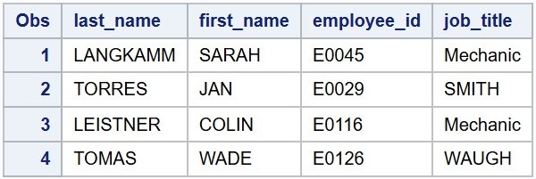
Now, let's read the same data file using the MISSOVER option:
DATA mydata.employees;INFILE '/home/u63368964/source/employees.dat' MISSOVER;INPUT last_name $ first_name $ employee_id $ job_title $;RUN;PROC PRINT DATA=mydata.employees;RUN;

When the MISSOVER option is used on the INFILE statement, the INPUT statement does not jump to the next line when reading a short line. Instead, MISSOVER sets variables to missing. In the printed out dataset, all lines are read in as separate row.
Notice, however, that the job_title are still missing for the sixth and seventh observation. This is because, while 37th to 45th column in the raw data file are designated for this variable, the value pilot does not fully extend to fill the entire width of the variable.
The TRUNCOVER option works similar to MISSOVER. However, when this option used instead of the MISSOVER option, SAS will take the partial values to fill the first unfilled variable. For example:
DATA mydata.employees;INFILE '/home/u63368964/source/employees.dat' TRUNCOVER;INPUT last_name $1-21 first_name $22-31 employee_id $32-36 job_title $37-45;RUN;PROC PRINT DATA=mydata.employees;RUN;

The INPUT Statement
After the INFILE statement, an INPUT statement must follow. This statement directs SAS on how to interpret the raw data by defining variables, their types (numeric or character), and their positions within the input record. In this section, we will explore the use of INPUT statements in various scenarios. Let's dive in!
Reading Raw Data Separated by Delimiters
List input (also called free formatted input) is a method for reading data into SAS when the values in your raw data file are all separated by one or more delimiters and each line in the file simply represents a single observation as a whole. If no DLM= option is specified in the INFILE statement, SAS uses spaces as the default delimiter. Otherwise, the raw data values must be separated by spaces when using list input.
List input is the most straightforward approach to read data. However, it has certain limitations:
- No skipping unwanted values: All data within a line must be read, even if some values are not needed.
- Missing data representation: Missing values must be represented by a period (.).
- Character data restrictions:
- Character data must be simple, with no embedded spaces.
- Maximum length for character variables is 8.
- Limited handling for formatted values: Raw data values should not be formatted in a specific way (e.g., $240,000 for a monetary value or Mar 19, 2024 for a date string).
Despite these restrictions, a surprisingly many number of data files can be read simply using the list input method.
To create an INPUT statement for list input, all you need to do is just listing the variable names in the same order as they appear in the data file. Make sure variable names are no longer than 32 characters long, start with a letter or an underscore (_), includes only letters, numerals, and underscores. For character variables, add a dollar sign ($) after the variable name. Lastly, make sure that there is at least one space between the variable names, and conclude the statement with a semicolon.
For example:
101 John 25 M 45000102 Sarah 29 F .103 Mike . . 48000104 Anna 31 F50000105 Bob . . .
This data may not appear very organized, but it satisfies all the requirements for list input: character data are 8 characters or fewer with no embedded spaces, all values are separated by at least one space, and missing data are represented by a period. Note that Anna's data continues onto the next line. This is not an issue because, by default, SAS will move to the next data line to read additional values if the number of variables in the INPUT statement exceeds the values available on the current line.
Here is the SAS program that will read the data:
DATA mydata.employees;INFILE '/home/u63368964/source/employees.dat';INPUT employee_id $ name $ age sex $ salary;RUN;PROC PRINT DATA=mydata.employees;RUN;

The variables employee_id, name, age, sex, and salary are listed after the INPUT keyword in the same order they appear in the data source. A dollar sign ($) following employee_id, name, and sex signifies that these are character variables. On the other hand, age and salary has no following dollar signs, meaning that they are numeric.
Reading Raw Data Arranged in Columns
In an INPUT statement, column indicators refer to the numbers placed after each variable name. These numbers maps the positions of the columns in the raw data file to each output variable, so that the output variables can be populated using the corresponding column values. For example, let's consider importing the raw data file saved as follows:
----+----1----+----2----+----3S001 John Doe 85 90 88S002 Jane Smith 92 88 95S003 Bob Johnson 78 82 80S004 Alice Lee 95 94 98S005 Emily Brown 80 85 82
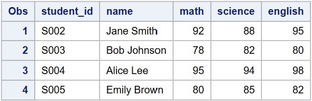
The following DATA step uses this file to create a new SAS dataset that includes the four variables: student_id, name, math, science, and english.
DATA mydata.student_grades;INFILE '/home/u63368964/source/student-grades.dat';INPUT student_id $ 1-4 name $ 6-20 math science english;RUN;PROC PRINT DATA=mydata.student_grades;RUN;
Here, the INPUT statement explicitly specifies raw data column ranges for each output variable. For example, any values in the 1-4 columns contained in the raw data file will be used to populate the student_id. Similarly, any values in the 6-20 columns will be used to the name. The remaining three variables are listed without column indicators, meaning that they assume that the values are separated by one or more spaces.
When the raw data file is well-organized in columns, using column indicators has several advantages over the default method:
- Character variables can contain spaces and have values of up to 32,767 characters.
- It's possible to skip values for unnecessary variables.
- Since the positions of columns to read are specified, they can be read in any order, and the same column can be read repeatedly.
For example, let's consider the following DATA step:
DATA mydata.student_grades2;INFILE '/home/u63368964/source/student-grades.dat';INPUT name $ 6-20 math science student_id $ 1-4 math_score 21-22;RUN;PROC PRINT DATA=mydata.student_grades2;RUN;
This DATA step reads raw data values from the 6th to the 20th columns of the raw data file and then creates the name variable for the student_grades2 SAS dataset. Then it moves to the next non-whitespace values to populate math. Similarly, it reads the next separated values to populate science. These two variables are created without column indicators. After that, SAS reads values in 1-4 columns of the same row, then populates student_id. Within the same row, SAS moves to the 21-22 columns again for another variable math_score.

Reading Raw Data Not in Standard Format
Sometimes raw data values are not straightforward numeric or character, and they may be in specific formats. For example, the value "1,000,001" includes commas to make it easier for humans to interpret as "one million and one". However, the embedded commas pose challenges when performing data imports, as computers interpret such values as a character string without any specific instructions.
The informats are used to guide SAS on how to interpret such "non-standard" [3] data values. Informats are useful anytime you have values like 1,000,001 or $45,000.00. Dates are perhaps the most common examples of non-standard data. For example, SAS converts conventional date formats like 10-31-2023 or 31OCT23 into the number of days since January 1, 1960. This number is known as a SAS date value.[4]
The three types of informats--character, numeric, and date--have the following forms:
$informatw. /* Character */informatw.d /* Numeric */informatw. /* Date */
Where w represents the total width, d indicates the number of decimal places (applicable only to numeric data), and the dollar sign ($) means a character informat. For example, let's consider the following raw data file:
----+----1----+----2----+----3----+----4-S001 01/05/2023 1,1250.00 Smartphone 0.20S002 01/06/2023 1,500.00 Laptop 2.50S003 01/07/2023 200.00 Headphones 0.10S004 01/08/2023 900.00 Tablet 0.80S005 01/09/2023 300.00 Smartwatch 0.15S006 01/10/2023 700.00 Camera 0.60S007 01/11/2023 150.00 Speaker 1.00S008 01/12/2023 400.00 Monitor 3.00S009 01/13/2023 50.00 Keyboard 0.50S010 01/14/2023 20.00 Mouse 0.20
The file above contains information on transaction ID, transaction date, transaction amount, product name, and product weights. Here, observe that each column has specific formats, such as MM/DD/YYYY for dates and comma-separated values for amounts. To read this data properly, we need informat specification in the INPUT statement as follows:
DATA mydata.sales;INFILE '/home/u63368964/source/sales.dat';INPUTtransaction_id $5.transaction_date MMDDYY11.transaction_amount COMMA10.2product_name $10.product_weight 4.2;RUN;PROC PRINT DATA=mydata.sales;RUN;
In this example, transaction_id $5. defines the character variable transaction_id by reading 5 column values from the input file. The width specification d is defined by 5 to fully extend the variable to the trailing space at the end. Similarly, MMDDYY11. instructs SAS to read the 11 values, such as 01/05/2023 including the trailing space, as SAS dates (the number of days between January 1, 1960 and January 5, 2023). The remaining three columns are also defined with their own informat specifications.

Here are some informats that are commonly used:
| Informat | Width | Input Data | INPUT Statement | Results |
|---|---|---|---|---|
| Character | ||||
| $CHARw. Reads character data, while preserving blanks. |
1-32767 (default: 8 or variable length) | John Doe Jane Doe |
INPUT name $CHAR10.; | John Doe Jane Doe |
| $UPCASEw. Converts character data to uppercase. |
1-32767 (default: 8) | John Doe | INPUT name $UPCASE10.; | JOHN DOE |
| $w. Reads character data, trimming leading blanks. |
1-32767 | John Doe Jane Doe |
INPUT name $10.; | John Doe Jane Doe |
| Date, Time, and Datetime | ||||
| ANYDATEw. Reads dates in various date forms. |
5-32 (default: 9) | 1jan1961 01/01/61 |
INPUT my_date ANYDATE10.; | 366 366 |
| DATEw. Reads dates in form: ddmmmyy or ddmmmyyyy |
7-32 (default: 7) | 1jan1961 1 jan 61 |
INPUT my_date DATE10.; | 366 366 |
| DATETIMEw. Reads dates in form: ddmmmyy hh:mm:ss.ss |
13-40 (default: 18) | 1jan1960 10:30:15 1jan1961,10:30:15 |
INPUT my_dt DATETIME18.; | 37815 31660215 |
| DDMMYYw. Reads dates in from: ddmmyy or ddmmyyyy |
6-32 (default: 6) | 01.01.61 02/01/61 |
INPUT my_date DDMMYY8.; | 366 367 |
| MMDDYYw. Reads dates in form: mmddyy or mmddyyyy |
6-32 (default: 6) | 01-01-61 01/01/61 |
INPUT my_date 8.; | 366 366 |
| JULIANw. Reads Julian dates in form: yyddd or yyyyddd |
5-32 (default: 5) | 61001 1961001 |
INPUT my_date JULIAN7.; | 366 366 |
| TIMEw. Reads time in form: hh:mm:ss.ss or hh:mm |
5-32 (default: 8) | 10:30 10:30:15 |
INPUT my_time TIME8.; | 37800 37815 |
| STIMERw. Reads time in form: hh:mm:ss.ss, mm:ss.ss, or ss.ss |
1-32 (default: 10) | 10:30 10:30:15 |
INPUT my_time STIMER8.; | 630 37815 |
| Numeric | ||||
| COMMAw.d Removes embedded commas and $. Converts values in parentheses to minus. |
1-32 (default: 1) | $1,000,000.99 (1,234.99) |
INPUT income COMMA13.2; | 1000000.99 -1234.99 |
| COMMAXw.d Similar to COMMAw.d, but switches role of comma and period. |
1-32 (default: 1) | $1.000.000,99 (1.234,99) |
INPUT income COMMAX13.2; | 1000000.99 -1234.99 |
| PERCENTw. Converts percentages to numbers. |
1-32 (default: 6) | 5% (20%) |
INPUT my_num PERCENT5.; | 0.05 -0.2 |
| w.d Reads standard numeric data. |
1-32 | 1234 -12.3 |
INPUT my_num 5.1; | 123.4 -12.3 |
Aside: Extracting Date Information from Numerals
Let's consider data like this:
2023 01 31 500000 350000 1500002023 02 28 520000 360000 1700002023 03 31 540000 370000 1700002023 04 30 530000 380000 1500002023 05 31 550000 390000 1600002023 06 30 560000 400000 1600002023 07 31 580000 410000 1700002023 08 31 600000 420000 1800002023 09 30 590000 415000 1750002023 10 31 610000 430000 1800002023 11 30 620000 440000 1800002023 12 31 650000 450000 200000
This data consists of space-separated values for year, month, day, revenue, expenses, and profit. When importing this data into a SAS dataset, importing the year, month, and day as separate numeric columns will prevent them from being recognized as dates. To preserve date information, you must create a new variable with SAS date values by combining the year, month, and day columns. This can be achieved using the MDY(month, date, year) function as shown below:
DATA month_end_closing;INFILE '/home/u63368964/source/month-end.dat';INPUT year month day revenue expenses profit;closing_date = MDY(month, day, year);RUN;PROC PRINT DATA=month_end_closing;RUN;
The MDY function returns a SAS date value from month, day, and year values. So, by using this function, we can convert the separate year, month, and day columns into a single SAS date variable, which can then be formatted and used for time-series analysis or any other date-related operations. Here is the PROC PRINT results:

Informat Modifiers
All three informats--character, numeric, and date--interpret raw data values according to the specified width. For example, $7. reads seven-character value such as Michael. However, in many cases, you might be unsure about the exact width of the values. While Michael fits perfectly into the $7., other values like Christopher for the same variable will be truncated. Similarly, a shorter value like Amy could result in part of the next column's values being read, causing incorrect data read.
For example, let's consider the following data file:
01 01 2020 Sedan Black 10 $25,00002 01 2020 SUV White 5 $25,00003 01 2020 Hatchback Red 8 $20,00004 01 2020 Sedan Blue 12 $26,00005 01 2020 Truck Gray 7 $40,00006 01 2020 SUV Silver 6 $36,00007 01 2020 Sedan Black 15 $25,50008 01 2020 Hatchback Blue 9 $20,50009 01 2020 SUV White 10 $35,50010 01 2020 Sedan Red 20 $26,000
Observe that the fourth and fifth columns (car model and color) have varying lengths. Now, let's run the following SAS program:
DATA mydata.car_sales;INFILE '/home/u63368964/source/car.dat';INPUT month day year model $15. color $15. num_sales msrp COMMA7.0;RUN;PROC PRINT DATA=mydata.car_sales;RUN;

Observe that the values are not imported correctly due to the varying length of the columns.
To import such values correctly, you should put a colon (:) in front of the column informats. This is called the colon modifier, which directs SAS to read the values up to the specified width, but stops at the first space (or other delimiter) it encounters.
DATA mydata.car_sales;INFILE '/home/u63368964/source/car-sales.dat';INPUT month day year model :$15. color :$15. num_sales msrp;RUN;PROC PRINT DATA=mydata.car_sales;RUN;

Let's consider another example. In the raw data file below, the first column (breeds) can possibly include a space. Thus, using colon modifier will not work, as it reads only up to the first space, leaving the remaining part of the value unread. For example, an informat specification like breeds :$50. will read the first observation as Labrador and truncate the remaining part of the value.
----+----1----+----2----+----3----+--Labrador Retriever 65 22 FriendlyGerman Shepherd 75 24 LoyalGolden Retriever 70 23 GentleBulldog 50 14 StubbornBeagle 25 15 EnergeticPoodle 45 22 IntelligentRottweiler 95 26 ConfidentYorkshire Terrier 7 7 BoldBoxer 70 25 PlayfulDachshund 11 8 CuriousSiberian Husky 60 23 IndependentDoberman Pinscher 75 26 Alert
To import this data file, you should use ampersand modifier. This modifier instructs SAS to treat a single space as part of a character variable, and two or more consecutive space characters are recognized as delimiters. In the raw data, observe that there are two spaces between the first and second column. So, putting an ampersand (&) right in front of the informat specification of the variable will successfully read the values.
DATA mydata.dog_breeds;INFILE '/home/u63368964/source/dogs.dat';INPUT breed &$50. avg_height avg_weight temper $;RUN;PROC PRINT DATA=mydata.dog_breeds;RUN;

Lastly, tilde modifier (~) instructs SAS to treat double quotation marks ("") as part of a variable's value. This modifier is commonly used alongside the DSD option in the INFILE statement. Remember that the DSD option tells SAS to ignore commas enclosed within quotation marks while removing the quotation marks themselves during import. However, when the DSD option is combined with the tilde modifier, SAS preserves the quotation marks, while recognizing the quoted strings as a single column value. For example, let's suppose that we want to import the data file below. In the process, we want to retain the quotation marks while ignoring the enclosed commas.
"Doe, John",25,Male,70,175"Smith, Alice",30,Female,55,160"Johnson, Bob",35,Male,80,180"Brown, Emily",28,Female,60,165"David, Michael",40,Male,85,185
To import this file, we can use a tilde modifier like below:
DATA mydata.height_weight;INFILE '/home/u63368964/source/height-weight.dat' DLM=',' DSD;INPUT name ~$15. age sex $ weight height;RUN;PROC PRINT DATA=mydata.height_weight;RUN;

Reading Messy Raw Data
Column Pointer Controls
Sometimes you need to read data that just don't line up in nice columns or have predictable lengths. In such cases, column indicators will not work and you have to use column pointers and colon modifiers.
- @n moves the cursor to n-th column.
- @'character string' moves the cursor right after the specified character string.
- +n moves the cursor to the n-th column after the current position.
For example, let's consider importing the following data file. This file contains information about temperatures for the month of July for Alaska, Florida, and North Carolina. Each line contains the city, state, normal high, normal low, record high, and the record low temperature in degrees Fahrenheit:
----+----1----+----2----+----3---CITY:Nome STATE:AK 5544 88 29CITY:Miami STATE:FL 9075 97 65CITY:Raleigh STATE:NC 8868 105 50
Now, let's consider the following DATA step:
DATA mydata.temp;INFILE '/home/u63368964/source/temperatures.dat';INPUT @'STATE:' state $@6 city $+10avg_high 2. avg_low 2.@27record_high record_low;RUN;PROC PRINT DATA=mydata.temp;RUN;
In the DATA step, @'STATE:' puts the column position, right after the given string 'STATE:', then reads data values until encounters a blank space. These values are assigned to the character variable state. Similarly, @6 relocates the current column position to the 6th column of the raw data file, and populates city.
Next, +10 moves the current position 3 columns after reading the value for the variable city. After reading the two subsequent variables, avg_high and avg_low, @27 locates the current position at the 27th column in the raw data and reads values for the remaining two variables.

Line Pointer Controls
Let's consider another example. This time, each observation spans three lines of the data file: the first line contains first and last name, second line contains age, and the third line contains height and weights.
David Shaw25189 90Amelia Serrano34165 61
Typically, each line of raw data represents one observation. However, in some cases, the data for a single observation is spread across multiple lines. SAS can automatically move to the next line if it runs out of data before reading all variables specified in the INPUT statement. While this default behavior works, it is better to explicitly instruct SAS when to move on the next line.
To control line transitions, you can use line pointers in your INPUT statement. Line pointers, slash (/) and pound-n (#n), serve as guides for SAS, directing it to the specified line of data. The slash pointer simply tells SAS to proceed to the next line, while #n pointer allows you to specify the exact line number within the observation. For example, #2 directs SAS to read from the second line of raw data, #4 refers to the fourth line. You can even go backwards using the #n pointer, reading from line 4 and then from line 3, for example. The slash is simpler, but #n is more flexible.
DATA mydata.height_weight;INFILE '/home/u63368964/source/height-weight.dat';INPUT first_name $ last_name $/ age#3 height weight;RUN;PROC PRINT DATA=mydata.height_weight;RUN;

Reading Multiple Observations per Line of Raw Data
By default, SAS assumes that each line of raw data corresponds to no more than one observation. When this is not the case, you can use double trailing at signs (@@) at the end of your INPUT statement. This line-hold specifier instructs SAS to "pause" and continue reading from the same line until either all data is processed or another INPUT statement without a double trailing @@ is encountered.
For example:
Laptop 999.99 5 Tablet 499.50 10 Phone 799.90 8Monitor 199.99 12 Keyboard 49.99 20 Mouse 25.50 15Headphones 149.99 7 Webcam 89.99 5 Speaker 129.99 10
Notice that each line contains multiple observations with three fields per observation: product, price and quantity. Now, the following program reads this data using @@:
DATA mydata.product_sales;INFILE '/home/u63368964/source/sales.dat';INPUT product $ price quantity @@;RUN;PROC PRINT DATA=mydata.product_sales;RUN;

Reading Part of a Raw Data File
Sometimes, you may need to extract a small subset of records from a large data source. For example, imagine you have a raw data like:
----+----1----+----2----+----3----+----4----+----5Inception 2010 Action 8.8 148Avengers 2012 Action 8.0 143Interstellar 2014 Adventure 8.6 169The Dark Knight 2008 Action 9.0 152Guardians of the Galaxy 2014 Action 8.1 121Stranger Things 2016 Adventure 8.7 50Breaking Bad 2008 Drama 9.5 62The Mandalorian 2019 Adventure 8.8 55The Witcher 2019 Action 8.2 60The Last of Us 2023 Adventure 9.1 45
Now, suppose that you want to create a SAS dataset, subsetting only those rows that are classified as "Action" and have rating above 8.0.
DATA mydata.action_above_8;INFILE '/home/u63368964/source/movies-tv-series.dat';INPUT title &$25. year genre $ rating @;IF genre ~= 'Action' OR rating <= 8.0 THEN DELETE;INPUT duration;RUN;PROC PRINT DATA=mydata.action_above_8;RUN;
In the DATA step shown above, observe that there are two INPUT statements. The first reads the variables: title, year, genre, and rating, and then ends with a trailing at sign (@). This instructs SAS to hold the current line of raw data during the subsequent IF statement checks if the value for genre is not 'Action' or rating is less than equal to 8.0. If it does, the second INPUT statement, reading the value for duration, will never executes.
Here is the result of the PRINT procedure:

Here is the full list of operators that you can use with the IF-THEN statement:
| Symbolic | Mnemonic | Example |
|---|---|---|
| = | EQ | WHERE name = 'John'; |
| ^=, ~=, <> | NE | WHERE name ^= 'John'; |
| > | GT | WHERE score > 80; |
| < | LT | WHERE score < 80; |
| >= | GE | WHERE score >= 80; |
| <= | LE | WHERE score <= 80; |
| & | AND | WHERE score >= 80 AND score <= 90; |
| |, ! | OR | WHERE name = 'John' OR name = 'Jane'; |
| IS NOT MISSING | WHERE score IS NOT MISSING; | |
| BETWEEN AND | WHERE score BETWEEN 80 AND 90; | |
| CONTAINS | WHERE name CONTAINS 'J'; | |
| IN (LIST) | WHERE name IN ('John', 'Jane'); |
Exporting and Downloading SAS Datasets
In SAS, "data exports" refers to the process of converting a SAS dataset file (*.sas7bdat) into external file formats, such as Excel (*.xlsx) or CSV (*.csv). This process allows data to be shared and used in applications outside of SAS. SAS Studio has point-and-click interface to do this.
- Navigate to "Libraries" section on the navigation pane.
- Right-click on the SAS dataset file that you want to export and select "Export". The Export Table window will appear.
- On the Export Table window, select where to store the exported dataset, specify proper file name, and select the output file format (e.g., *.xlsx, *.csv, etc.).
- Click "Export".

The exported data file will be stored within the cloud environment of SAS Studio. To download the exported file to your local machine, go to "Server Files and Folders" section, right-click on the file, and select "Download File".


0 Comments