

DATA Step's Implicit Loop
In our previous tutorial, we explored how to create a new SAS dataset using DATA step. A key component of this process is the INFILE statement, which tells SAS where to read the incoming raw data values. As the DATA step executes, each row from the external file is read, processed, and added to the SAS dataset.
Let's take a closer look at what happens behind the scenes.
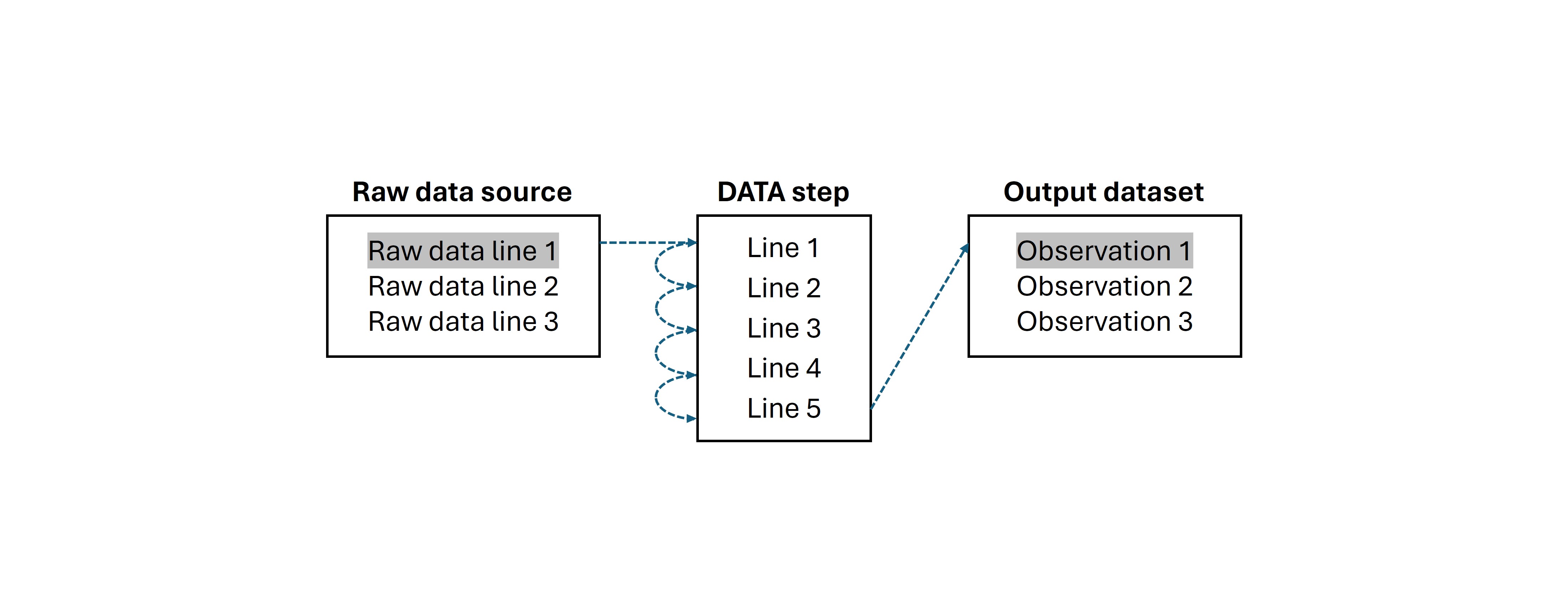
When you submit a DATA step, SAS first initializes a temporary structure called as the Program Data Vector (PDV). Think of the PDV as a staging area--a workplace where SAS builds each observation one row at a time. As the DATA step runs, values from the current row are loaded into the PDV and manipulated according to your instructions.
Once all statements for that row are executed, the contents of the PDV are written to the output dataset as a new observation. SAS then clears the PDV and repeats the process for the next row. This cycle continues until all rows from the input source have been processed. This repetitive mechanism is known as the DATA step's implicit loop.
For example, consider the following text file containing sales transaction data:
1 2023-11-01 WidgetA 10 100.002 2023-11-01 WidgetB 5 75.003 2023-11-02 WidgetA 8 80.004 2023-11-02 WidgetC 15 150.005 2023-11-02 WidgetB 12 180.00
Suppose that you want to create a SAS dataset from this file, including six variables: transaction_id, date, product, quantity, unit_price, and sales_amount.
Here's how you can do it using a DATA step:
DATA mydata.sales;INFILE '/home/u63368964/source/sales.txt';INPUT transaction_id $ date :yymmdd10. product $ quantity unit_price;sales_amount = quantity * unit_price;RUN;
When this DATA step runs, SAS performs the following actions:
- Initialize PDV: SAS creates a temporary workspace to hold values for each row from the data source.
- Reads and Assign Values: The INPUT statement reads the first five values--1, 2023-11-01, WidgetA, 10, and 100.00--and loads them into the PDV. Then, it assigns each value to its proper variable.
- Calculates Derived Variable: The next statement computes sales_amount by multiplying quantity and unit_price of the current row.
- Writes to Dataset: After all statements for the current row are executed, SAS writes the contents of the PDV to the output dataset as a new observation.
This process repeats for each line in the text file, resulting in five observations in the final dataset mydata.sales.
While the inner workings of the DATA step might seem like technical jargon at first, understanding what's going on behind the scene is incredibly useful for feature engineering in SAS. Because the loop processes each row individually, it allows you to create new variables, apply conditional logic, and transform data on a row-by-row basis--all within a single DATA step. This makes it easy to derive features like calculated metrics, indicator flags, or categorical groupings directly from raw input, streamlining the path from raw data to analytical-ready datasets.
Assignment Statement and Expressions
Creating a new variable for the output dataset in a DATA step is straightforward. You can easily do this using the assignment operator (=):
new-variable = expression;
This is called the assignment statement. When you run a DATA step, SAS processes each row of the reference data by loading its value into the PDV, executing the assignment statements to populate the PDV, and then appending the values from the PDV as an observation in the output dataset.
On the left side of the equal sign should be the variable name, which can be either a new one, to append one more variable to the data set, or existing one, to re-define it by the expression. Naming rules for the variables are:
- SAS variable names can be up to 32 characters in length.
- The first character must begin with an English letter or an underscore (_).
- Subsequent characters can be English letters, numeric digits, or underscores.
- A variable name cannot contain any special characters (e.g., blank spaces, @, !, etc.) other than the underscore.
- SAS reserves a few names for automatic variables (e.g., _N_ and _ERROR_).
On the right side of the equal sign should be an expression like:
| Expressions | Description | Example |
|---|---|---|
| Numeric constant | Assigns the value 10 to each observation of the variable x. | x = 10; |
| Character constant | Assigns the character string "John" to each observation of the variable name. | name = "John"; |
| New variable | Assigns each observation of old_var to the corresponding observation of new_var. | new_var = old_var; |
| Addition | Assigns the sum of each row's values in num1 and num2 to the corresponding observation of the variable total. | total = num1 + num2; |
| Subtraction | Assigns the result of subtracting num2 from num1 to the variable difference. | difference = num1 - num2; |
| Multiplication | Assigns the multiplication of num1 and num2 to the variable product. | product = num1 * num2; |
| Division | Assigns the result of dividing num1 by num2 to the variable division. | division = num1 / num2; |
| Exponentiation | Assigns the 10th power of num1 to the variable power. | power = num1 ** 10; |
| Concatenation | Assigns the concatenation of two character variables to the new variable full_name. | full_name = first_name || last_name; |
Feature Engineering in SAS DATA Step
Feature engineering is the process of creating, transforming, or selecting variables that help a data model or analysis better understand patterns in the data. These new variables serve as the foundation for predictive modeling, classification, clustering, and other analytical tasks.
In a typical workflow, when a company collects raw data from its business--such as transactional systems, web logs, or IoT devices--it stores that data in a centralized repository called a data warehouse. Data engineers then clean, standardize, and integrate this raw data to ensure consistency and usability. Following that, feature engineering takes over. Analysts and data scientists derive new variables from the cleaned data--such as ratios, flags, time-based indicators, or aggregated metrics--that are tailored to specific business questions or modeling goals.
These curated datasets are then organized into data marts: subject-specific subsets of the data warehouse designed for analysis. A data mart contains analysis-ready data, enriched in engineered features that accelerate insights and improve model performance.

Once the foundational data is cleaned and stored in a data warehouse, feature engineering strategies used to build data marts generally fall into two broad categories: row-level transformations and group-level summarized metrics.
- Row-Level Operations: These involve deriving features by transforming or combining existing variables within individual rows. Deriving new features by row-level operations are ideal for granular analysis and predictive modeling, but it requires strong domain knowledge and must be backed by robust logic to ensure relevance and accuracy.
- Group-Level Summaries: These features are created by aggregating data across multiple rows, typically grouped by a key such as customer ID, product category, or time period. Group-level metrics help capture behavioral trends, perfor
prepared,
, it stores it in a centralized repository called a data warehouse. Then, the company creates new variables using feature engineering and compose data mart. The data mart is analysis ready datasets.
In general, when a company first collects raw data, they make data mart
Let's consider an example scenario. According to fitness experts, the one-repetition maximum (one-rep max or 1RM) in weight training refers to the maximum weight an individual can possibly lift for a single repetition. Based on the past workout logs, there are several ways to calculate 1RM:
- Epley Formula: 1 RM \(= \text{Weight Lifted} \times (1 + 0.0333) \times \text{Number of Reps}\)
- Brzycki Formula: 1 RM \(= \frac{\text{Weight Lifted}}{1.0278 - 0.0278 \times \text{Number of Reps}}\)
- Lombardi Formula: 1 RM \(= \text{Weight Lifted} \times \text{Number of Reps}^{\frac{1}{10}}\)
- O'Conner Formula: 1 RM \(= \text{Weight Lifted} \times (1 + 0.025) \times \text{Number of Reps}\)
The following DATA steps perform different 1RM calculations using reps and weights:
DATA workout_log;INPUT timestamp :DATETIME. exercise :$50. reps sets weights;/* Creating new variables */epley = weights * (1 + 0.0333 * reps); brzycki = weights / (1.0278 - 0.0278 * reps); lombardi = weights * reps ** 0.1; oconner = weights * (1 + 0.025 * reps);DATALINES;27MAR2023:08:00:00 Squats 10 3 10027MAR2023:08:15:00 Push-ups 15 3 .27MAR2023:08:30:00 Bench-press 8 4 12027MAR2023:08:45:00 Deadlifts 12 3 15027MAR2023:09:00:00 Lunges 10 3 8027MAR2023:09:15:00 Pull-ups 8 4 027MAR2023:09:30:00 Bicep-curls 12 3 4027MAR2023:09:45:00 Planks . . .27MAR2023:10:00:00 Shoulder-press 10 3 50;RUN;PROC PRINT DATA=workout_log;RUN;
For mathematical expressions, SAS follows the standard order of operations: exponentiation first, then multiplication and division, followed by addition and subtraction. Parentheses override the order; any calculations within the parentheses are performed first.
If any missing value is involved in a mathematical operation, the calculation will also result in a missing value. You can check if there were any missing value involve in the calculation by reviewing the log:
For example, in the dataset above, the second observation has a missing value for weights. So, if you run this DATA step, the four variables--epley, brzycki, lombardi, and oconner--will be missing.

One trick to avoid this is using the SUM function like:
DATA workout_log;INPUT timestamp :DATETIME. excercise :$50. reps sets weights;/* Creating new variables */epley = SUM(weights, 0) * (1 + 0.0333 * reps); brzycki = SUM(weights, 0) / (1.0278 - 0.0278 * reps);lombardi = SUM(weights, 0) * reps ** 0.1;oconner = SUM(weights, 0) * (1 + 0.025 * reps);DATALINES;27MAR2023:08:00:00 Squats 10 3 10027MAR2023:08:15:00 Push-ups 15 3 .27MAR2023:08:30:00 Bench-press 8 4 12027MAR2023:08:45:00 Deadlifts 12 3 15027MAR2023:09:00:00 Lunges 10 3 8027MAR2023:09:15:00 Pull-ups 8 4 027MAR2023:09:30:00 Bicep-curls 12 3 4027MAR2023:09:45:00 Planks . . .27MAR2023:10:00:00 Shoulder-press 10 3 50;RUN;PROC PRINT DATA=workout_log;RUN;
In this example, observe that the SUM function is used to add 0 to each value of the variable weights. This ensures that if weights is missing, the SUM function will return 0. Consequently, the subsequent calculations will be performed using 0 instead of the missing value.
.jpeg)
Selected Functions for Handling Numeric and Character Data
In addition to the operators discussed earlier, SAS offers a wide range of built-in functions for processing numeric and character data.[1] The table below provides a summary of commonly used functions.
| Function | Description | Example | Result |
|---|---|---|---|
| Numeric | |||
| ROUND(x, int) | Rounds a numeric value to a specific number of decimals. | ROUND(3.141592, 2) | 3.14 |
| INT(x) | Returns the integer part of x, by truncating any fractional digits. | INT(3.75) INT(-2.1) | 3 -2 |
| ABS(x) | Returns the absolute value of x. | ABS(-5) | 5 |
| CEIL(x) | Returns the smallest integer that is greater than or equal to x. | CEIL(4.3) CEIL(-1.5) | 5 -1 |
| FLOOR(x) | Returns the largest integer that is less than or equal to x. | FLOOR(4.8) FLOOR(-1.5) | 4 -2 |
| LOG(x) | Returns the natural logarithm of x (base-e logarithm). | LOG(10) | 2.302585 |
| EXP(x) | Returns the base-e raised to the power of x. | EXP(1) | 2.71828 |
| SQRT(x) | Returns the square root of x. | SQRT(9) | 3 |
| MOD(dividend, divisor) | Returns the remainder after dividing two numbers. | MOD(5, 3) | 2 |
| MAX(arg1, arg2, ...) | Returns the maximum value among the arguments. | MAX(5, 10, 3) | 10 |
| MIN(arg1, arg2, ...) | Returns the minimum value among the arguments. | MIN(5, 10, 3) | 3 |
| SUM(arg1, arg2, ...) | Calculates the sum of the arguments. Missing values are ignored. | SUM(5, 10, 3) SUM(0, 1, .) | 18 1 |
| MEAN(arg1, arg2, ...) | Calculates the average of the arguments. Missing values are ignored. | MEAN(5, 10, 3) MEAN(1, 2, ., 3) | 6 2 |
| Character | |||
| ANYALNUM(arg, start) | Returns position of first occurrence of any alphabetic character or numeral at or after optional start position. | a='123 E St, #2 '; x=ANYALNUM(a); y=ANYALNUM(a,10); | x=1 y=12 |
| ANYALPHA(arg, start) | Returns position of first occurrence of any alphabetic character at or after optional start position. | a='123 E St, #2 '; x=ANYALPHA(a); y=ANYALPHA(a,10) | x=5 y=0 |
| ANYDIGIT(arg, start) | Returns position of first occurrence of any numeral at or after optional start position. | a='123 E St, #2 '; x=ANYDIGIT(a); y=ANYDIGIT(a,10) | x=1 y=12 |
| ANYSPACE(arg, start) | Returns position of first occurrence of a white space character at or after optional start position. | a='123 E St, #2 '; x=ANYSPACE(a); y=ANYSPACE(a,10) | x=4 y=10 |
| CAT(arg-1, arg-2, ... arg-n) | Concatenates two or more character strings together leaving leading and trailing blanks. | a=' cat'; b='dog '; x=CAT(a,b); y=CAT(b,a); | x=' catdog ' y='dog cat' |
| CATS(arg-1, arg-2, ... arg-n) | Concatenates two or more character strings together stripping leading and trailing blanks. | a=' cat'; b='dog '; x=CATS(a,b); y=CATS(b,a); | x='catdog' y='dogcat' |
| CATX('separator-string', arg-1, arg-2, ... arg-n) | Concatenates two or more character strings together stripping leading and trailing blanks and inserting a separator string between arguments. | a=' cat'; b='dog '; x=CATX('&',a,b); | x='cat&dog' |
| COMPRESS(arg, 'char') | Removes spaces or optional characters from argument. | a=' cat & dog '; x=COMPRESS(a); y=COMPRESS(a,'&'); | x='cat&dog' y=' cat dog ' |
| INDEX(arg, 'string') | Returns starting position for string of characters. | a='123 E St, #2 '; x=INDEX(a,'#') | x=11 |
| LEFT(arg) | Left aligns a SAS character expression. | a=' cat'; x=LEFT(a); | x='cat ' |
| LENGTH(arg) | Returns the length of an argument not counting trailing blanks (missing values have a length of 1). | a='my cat'; b=' my cat '; x=LENGTH(a); x=LENGTH(b); | x=6 y=7 |
| PROPCASE(arg) | Converts first character in word to uppercase and remaining characters to lowercase. | a='MyCat'; b='TIGER'; x=PROPCASE(a); y=PROPCASE(b); | x='Mycat' y='Tiger' |
| SUBSTR(arg, position, n) | Extracts a substring from an argument starting at position for n characters or until end if no n. | a='(916)734-6281'; x=SUBSTR(a,2,3); | x='916' |
| TRANSLATE(source, to-1, from-1, ... to-n, from-n) | Replaces from characters in source with to characters (one to one replacement only - you can't replace one character with two, for example). | a='6/16/99'; x=TRANSLATE (a,'-','/'); | x=6-16/99 |
| TRANWRD(source, from, to) | Replaces from character string in source with to character string. | a='Main Street'; x=TRANWRD (a,'Street','St.'); | x='Main St.' |
| TRIM(arg) | Removes trailing blanks from character expression. | a='My '; b='Cat'; x=TRIM(a)||b; | x='MyCat' |
| UPCASE(arg) | Converts all letters in argument to uppercase. | a='MyCat'; x=UPCASE(a) | x='MYCAT' |
It is worth noting that, when used in an assignment statement, the functions listed above perform element-wise calculations across variables for each observation, not across observations for a variable. This is because, just like the execution of any other DATA step statements, the assignment statement operates on each row values in the current PDV in the DATA step's internal loop. For example:
DATA mydata;INPUT var1 var2 var3;/* Element-wise calculation within an observation */total = SUM(var1, var2, var3);avg = MEAN(var1, var2, var3);DATALINES;10 20 305 15 258 12 18RUN;PROC PRINT DATA=mydata;RUN;
.jpeg)
Observe that the calculation is performed across variables, not across observations.
Working with Dates
In SAS, date values are represented as the number of days since January 1, 1960. For example, January 1, 1959 is -365, January 1, 1961 is 366 (due to the leap year), January 1, 1960 is 0, and January 1, 2020 is 21915. This representation makes date calculations easier in most cases, as you can directly add or subtract the date values. For example, if a library book is due in three weeks, you could find the due date by adding 21 days to the date it was checked out.
DATA _null_;checkout_date = '01JAN2020'd;due_date = checkout_date + 21;PUT due_date date9.; /* Display the due_date in the SAS log */RUN;
You can use a date as a constant in a SAS expression by formatting it in the DATEw. (e.g., 01Jan2020). Then, enclose the date in quotation marks followed by a letter 'd'. The assignment statement above creates a variable named checkout_date, which is assigned the SAS date value for January 1, 2020.
In addition to the arithmetic expressions, SAS also has built-in functions to perform a number of handy operations. Here are some selected date functions:
| Functions | Description | Example | Result |
|---|---|---|---|
| DATEJUL(julian-date) | Converts a Julian date to a SAS date value. | DATEJUL(60001) DATEJUL(60365) |
0 364 |
| MDY(month, day, year) | Returns a SAS date value from month, day, and year values. | MDY(1,1,1960) MDY(2,1,60) |
0 31 |
| YEAR(date) | Returns year from a SAS date value. | YEAR('04DEC2023'd) YEAR(MDY(7,31,1962)) |
2023 1962 |
| QTR(date) | Returns the yearly quarter (1-4) from a SAS date value. | QTR('04DEC2023'd) QTR(MDY(7,31,1962)) | 4 3 |
| MONTH(date) | Returns the month (1-12) from a SAS date value. | MONTH('04JAN2024'd) MONTH(MDY(12,1,1960)) |
1 12 |
| DAY(date) | Returns the day of the month from a SAS date value. | DAY('04JAN2024'd) DAY(MDY(4,18,2012)) |
4 18 |
| WEEKDAY(date) | Returns day of week (1=Sunday) from SAS date value. | WEEKDAY('04JAN2024'd) DAY(MDY(4,13,2012)) | 5 6 |
| TODAY() | Returns the current date as a SAS date value. | TODAY() |
System date |
| YRDIF(start, end, 'AGE') | Computes difference in years between two SAS date values taking leap years into account. | YRDIF('23NOV1991'd, '04JAN2024'd, 'AGE') | 32.115068493 |
When encountering a two-digit year (e.g., 07/04/34), SAS needs to determine the correct century. Is it 1934 or 2034? The system option YEARCUTOFF= specifies the starting year of the default century range for SAS. To modify this default setting, use the OPTIONS statement like below:
OPTIONS YEARCUTOFF = 1950;
This statement sets two-digit dates as occurring between 1950 and 2049.
Aside: Using Shortcuts for List of Variable Names
Let's be honest, typing out long lists of variables in SAS can get pretty tiring. Imagine a DATA step with 100 variable assignments. By the time you reach the 49th variable, you're probably ready to throw in the towel! Thankfully, there are easier ways to handle this.
Numbered Range Lists
A series of variables that share the same name except for consecutive numbers at the end can be represented using a numbered range list. The sequence of numbers can start and end anywhere within the range, as long as all numbers between them are included. For example, the following INPUT statement shows a variable list and its abbreviated form:
- Variable List: INPUT var3 var4 var5 var6 var7;
- Abbreviated List: INPUT var3 - var7;
Name Prefix Lists
Prefixed variables can be grouped using a name prefix list. For example:
- Variable List: SUM(sales_electronics, sales_clothing, sales_groceries);
- Abbreviated List: SUM(OF sales_:);
Name Range Lists
Name range lists are based on the internal order, or position, of the variables in the SAS dataset. This internal order is determined by the order in which the variables appear in the DATA step. For example, consider the following DATA step:
DATA example;INPUT x y;z = x + y;RUN;
In this case, the internal variable order would be x, y, z.
The abbreviated list of variables can be used almost anywhere in a SAS program. When used as arguments for functions, however, remember to include the keyword OF before the abbreviated list (e.g., SUM(OF var1 - var100)). In other cases, simply replace the manually typed list of variables with the abbreviated list.
Feature Engineering in a SAS DATA Step
The performance of many statistical models and machine learning algorithms heavily rely on how variables (or features, in machine learning terminology) can effectively extract the key information from the data. Depending on your data and analysis purpose, there are many different techniques for feature engineering. In image recognition, for example, the convolutional layers of a CNN model captures spatial patterns in the image, such as edges, textures, and shapes, which are essential information for identifying objects. Similarly, in natural language processing tasks, techniques like word embeddings (e.g., Word2Vec or GloVe) transform text data into numeral vectors, enabling the representation of semantic relationships between words in a numeral format.
SAS is mainly designed for working with tabular data, where data values are organized by rows and columns. In the context of tabular data, common feature engineering techniques include:
- Binning: Grouping continuous variables into discrete categories.
- Encoding: Converting categorical variables into numeral representations.
- Standardizing: Transforming variables to have a mean of 0 and a standard deviation of 1.
All these processes of selecting, extracting, and transforming variables are collectively known as feature engineering. In the following subsections, we'll explore how to perform the three most common feature engineering techniques in a SAS DATA step. Let's get started!
Using IF-THEN Statements for Binning and Encoding
Binning is the process of grouping continuous variables into discrete categories or intervals. It is a very common technique in data preprocessing, where numeral data is divided into bins or ranges, which can mitigate the impact of outliers by grouping extreme values together and reduce noise in the data.
In a SAS DATA step, you can achieve this using the IF-THEN statement.
IF <condition> THEN <action>;
If condition evaluated to be true, then SAS executes action. Here are operators that can be used in the condition part:
| Symbolic | Mnemonic | Example |
|---|---|---|
| = | EQ | WHERE name = 'John'; |
| ^=, ~=, <> | NE | WHERE name ^= 'John'; |
| > | GT | WHERE score > 80; |
| < | LT | WHERE score < 80; |
| >= | GE | WHERE score >= 80; |
| <= | LE | WHERE score <= 80; |
| & | AND | WHERE score >= 80 AND score <= 90; |
| |, ! | OR | WHERE name = 'John' OR name = 'Jane'; |
| IS NOT MISSING | WHERE score IS NOT MISSING; | |
| BETWEEN AND | WHERE score BETWEEN 80 AND 90; | |
| CONTAINS | WHERE name CONTAINS 'J'; | |
| IN (LIST) | WHERE name IN ('John', 'Jane'); |
For example:
DATA employees;INPUT name $ job_title &$15. salary work_hours;DATALINES;John Statistician I 50000 40Sara Statistician I 60000 45Mike Statistician II 45000 38Alice Statistician I 80000 42David Statistician I 100000 48Eva Statistician II 70000 40James Statistician I 120000 50Sophia Statistician II 75000 42Michael Statistician II 85000 45Olivia Statistician I 1800000 70RUN;PROC MEANS DATA=employees;TITLE 'Salary Statistics';VAR salary;RUN;

In this example, observe that one salary value has an extreme value, which heavily affects the mean salary, making it less representative for the majority of the other salaries in the dataset.
To address this, you can organize the salary data into groups as shown below:
DATA grouped_salaries;SET employees;IF salary <= 60000 THEN DO;salary_class = '45,000-60,000';class_mark = (45000 + 60000) / 2;END;ELSE IF salary > 60000 AND salary <= 77500 THEN DO;salary_class = '60,000-77,500';class_mark = (60000 + 77500) / 2;END;ELSE IF salary > 77500 AND salary <= 100000 THEN DO;salary_range = '77,500-100,000';class_mark = (77500 + 100000) / 2;END;ELSE IF salary > 100000 THEN DO;salary_range = '100,000-1,800,000';class_mark = (100000 + 1800000) / 2;END;RUN;PROC FREQ DATA=grouped_salaries;TABLE salary / OUT=freq_table;RUN;
A single IF-THEN statement can only have one action. To execute more than one actions under a condition, you need to enclose the actions within DO and END statements. For example, when the condition salary <= 60000 turns out to be true for an observation, SAS performs two actions: it assigns the value '45,000-60,000' to the variable salary_class and calculates class_mark variable as (45000 + 60000) / 2.
The DO statement ensures that all SAS statements following it are treated as a single unit until a matching END statement is encountered. Together, the DO statement, the END statement, and all statements in between form what is known as a DO group.
Here is the PROC FREQ result:

This result is saved as a separate dataset named freq_table, as specified in the OUT= option in the TABLE statement. The dataset can then be used to calculate the average salary based on the class mark, mitigating the impact of extreme values.
Encoding a categorical variable involves converting categorical data into a numerical format suitable for analysis or machine learning models (e.g., "Statistician II" = 0 and "Statistician I" = 1). In a SAS DATA step, encoding can be done using the IF-THEN statements like below:
DATA encoded_jobs;SET employees;IF job_title = 'Statistician I' THEN job_code = 0;ELSE job_code = 1;RUN;PROC FREQ DATA=encoded_jobs;TITLE 'Encoded Job Titles';TABLE job_code;RUN;

Aside: Subsetting IF
The IF-THEN statement can also be used to create a subset of an existing dataset. For example:
DATA employee_subset;SET employees;IF salary >= 100000 THEN DELETE;RUN;PROC PRINT DATA=employee_subset;RUN;

Standardizing Data
Data standardization is the process of transforming variables to have a common scale, usually with a mean of zero and a standard deviation of one. This technique is particularly useful when working with data that has different units or ranges, as it helps ensure that each variable contributes equally to statistical analyses or machine learning models.
To goal of standardization is to make the data more comparable across variables. For example, if one variable represents height in centimeters and another represents income in thousands of dollars, the difference in scales between these two variables could impact the results of a model. Standardization removes this issue by scaling the data to a common range.
Formula for Standardization
Standardization is typically done using the following formula for each data point:
\(z = \frac{X - \mu}{\sigma}\)
Where:
- \(X\) is the original value.
- \(\mu\) is the mean of the variable.
- \(\sigma\) is the standard deviation of the variable.
- \(z\) is the standardized value.
For example, in the employees dataset, the summary statistics for salary and work_hours are as follows:
PROC MEANS DATA=employees;VAR salary work_hours;RUN;

Now, using the statistics, you can standardize the two variables as follows:
DATA z_scores;SET employees;z_salary = (salary - 248500) / 545603;z_work_hours = (work_hours - 46) / 9.2255683;RUN;PROC PRINT DATA=z_scores;RUN;

The standardized values can later be used to perform:
- Statistical Analysis: In methods like principal component analysis (PCA), standardization is necessary because the algorithm uses variances, which can be affected by the scale of features.
- Machine Learning Algorithms: Many algorithms (e.g., k-nearest neighbors, supported vector machines) assume that all features have the same scale. Even when data standardization is not required, using standardized features enhances model performance. For example, neural networks tend to perform better when input data is standardized, as it helps with faster convergence during training.
Aside: The RETAIN Statement and Automatic Variables
By default, when SAS completes all DATA step statements for the current observation, the values in the PDV are reset to be empty. However, if a RETAIN statement is used in the DATA step with a specific variable with an assigned value, the corresponding PDV element retains the specified value.
To understand how it works, it is best to use a practical example. The sashelp.gnp dataset has quarterly data on national economy from 1960 to 1991.

Where:
- GNP: Gross national product (in billions of dollars)
- CONSUMP: Personal consumption expenditures
- INVEST: Gross private domestic investment
- EXPORTS: Net exports of goods and services
- GOVT: Government purchases of goods and services
Now, suppose that you want to track the record high and record low for personal consumption expenditures. This can be achieved by:
DATA consumption_records;/* Bring data from mydata.gnp */SET sashelp.gnp;/* Track high and low of consump in the record_high and record_low */ RETAIN record_high 0; record_high = MAX(record_high, consump);RETAIN record_low;record_low = MIN(record_low, consump); RUN;/* First 20 consumption expenditures */PROC PRINT DATA=consumption_records (OBS=20);VAR date consump record_high record_low;RUN;
When processing the first observation, RETAIN record_high 0; initializes the new variable record_high with a value of 0. In the following line of code, MAX(record_high, consump) compares the current record_high value (0) with the consump value from the first observation (325.5). The code then assigns the larger of the two values, in this case, 325.5, to record_high. This value is retained for the next observation.
When processing the second observation, record_high = MAX(record_high, consump); compares the updated record_high (325.5) with the consump from the second observation (331.6). Since 331.6 is greater than 325.5, record_high is updated to 331.6. This process continues for each subsequent observation, ensuring that record_high always reflects the highest consump value encountered so far.
Similarly, RETAIN record_low; instructs SAS to retain the value of record_low from the previous observation to the current observation. Observe that the record_low is initialized without specific value. By default, SAS initializes retained variables without an explicit value to a missing value.
Here is the first 20 observation of the output dataset:

This time, suppose you want to calculate quarter-on-quarter (QoQ) growth rate of the GNP. To calculate QoQ, substract the previous quarter's GNP value from the current quarter's value, divide the result by the previous quarter's value, and then multiply by 100:
\(QoQ = \frac{\text{Current Quarter's GNP} - \text{Previous Quarter's GNP}}{\text{Previous Quarter's GNP}} \times 100%\)
To achieve this, you can use the following approach:
DATA qoq_gnp;SET sashelp.gnp;RETAIN gnp_prev;diff = gnp - gnp_prev;qoq = (diff / gnp_prev) * 100;/* Update gnp_prev by gnp */gnp_prev = gnp;RUN;PROC PRINT DATA=qoq_gnp (OBS=20);VAR date gnp diff qoq;RUN;
In this DATA step, the RETAIN statement initializes gnp_prev with a missing value and retains the current value for the next iteration. Since gnp_prev is missing for the first observation, the subsequent assignments (diff = gnp - gnp_prev; and qoq = (diff / gnp_prev) * 100;) will also be missing for the observation. Then gnp_prev = gnp; updates the gnp_prev variable with the current quarter's GNP value, preparing it for the calculation in the next observation. So, when processing the second observation, for example, the diff and qoq will be calculated based on the stored value in the gnp_prev at the moment.
Here is the first 20 observations of the output dataset:

Next, suppose that you want to calculate the running totals of the investments. To calculate the running total:
DATA total_invest;SET sashelp.gnp;RETAIN running_total invest;running_total = SUM(running_total, invest);[2] RUN;PROC PRINT DATA=total_invest;VAR date invest running_total;RUN;

Now, let's also calculate the yearly total investments. This requires reset of the total investments for every four quarters. You can achieve this as follows:
DATA yearly_invest;SET sashelp.gnp;/* Initialize running_total and yearly_total by invest */RETAIN running_total invest yearly_total invest;/* Calculate running_total */running_total = SUM(running_total, invest);/* Calculate yearly_total */IF MOD(_N_, 4) = 1 THEN yearly_total = invest;ELSE yearly_total = SUM(yearly_total, invest); RUN;PROC PRINT DATA=yearly_invest (OBS=20);VAR date invest running_total yearly_total;RUN;
In the DATA step, the condition IF MOD(_N_, 4) = 1 checks if the remainder is 1 when the current observation number (_N_) is divided by 4. If it is, meaning the first quarter of the year, then the yearly_total is set to the current value of the invest. Otherwise, yearly_total is set to the sum of the previous value of yearly_total and the current invest.
Here is the first 20 observations of the output dataset:

In SAS, automatic variables are special system variables that are created and maintained automatically by the DATA step. They provide information about the current status from the DATA step's internal loop and can be used within your code.
Here is the list of the automatic variables:
- _N_: Holds the current observation number in the DATA step's internal loop. It starts at 1 and increments by 1 with each observation processed.
- _ERROR_: If there is an error for the current observation, _ERROR_ will be set to 1; otherwise, it will be 0.
- FIRST.variable and LAST.variable: These two are created for each BY variable and indicate if the observation is the first and last for the BY group.
Generally, automatic variables exist temporarily only during the execution of the current DATA step and are not stored as part of the output dataset. So, if you want to include the automatic variables in your output, you should explicitly assign them:
DATA yearly_invest;SET sashelp.gnp;RETAIN running_total invest yearly_total invest;running_total = SUM(running_total, invest);IF MOD(_N_, 4) = 1 THEN yearly_total = invest;ELSE yearly_total = SUM(yearly_total, invest);/* Assigning _N_ to n_obs */n_obs = _N_; RUN;PROC PRINT DATA=yearly_invest (OBS=20);VAR n_obs date invest running_total yearly_total;RUN;

When the BY statement is used in a DATA step (typically for combining two datasets using the SET, MERGE, or UPDATE statements or grouping data by the BY group), FIRST.variable and LAST.variable are available. FIRST.variable will have a value of 1 when SAS encounters an observation with the first occurrence of a new value for that variable, and 0 for the other observations. Similarly, LAST.variable will have a value of 1 for an observation with the last occurrence of a value for that variable, and 0 for the other observations. For example:
DATA sales_data;INPUT region $ sales;DATALINES;North 100North 200North 150South 300South 400East 250;DATA region_totals;SET sales_data;/* Group data by retion */BY region NOTSORTED;[3]/* Initialize total at the start of each region */IF first.region THEN total_sales = 0;/* Accumulate sales */total_sales + sales;RUN;PROC PRINT DATA=region_totals;RUN;

[1] In SAS, dates are saved as SAS date values, which is the number of days since January 1, 1960. So, essentially, they are just integers. This turns out to be extremely useful for date calculations. For example, you can easily find the number of days between two dates by simply subtracting one date value from the other. ↩


0 Comments